Download
1 / 25
250 likes | 505 Views
Learn the concept of random variables and types of probability distributions. Explore examples and calculations for discrete and continuous random variables.

E N D
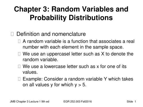
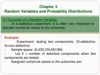
Chapter 3 Random Variables and Probability Distributions 3.1 Concept of a Random Variable: · In a statistical experiment, it is often very important to allocate numerical values to the outcomes. Example: · Experiment: testing two components. (D=defective, N=non-defective) · Sample space: S={DD,DN,ND,NN} · Let X = number of defective components when two components are tested. · Assigned numerical values to the outcomes are:
Notice that, the set of all possible values of the random variable X is {0, 1, 2}. Definition 3.1: A random variable X is a function that associates each element in the sample space with a real number (i.e., X : SR.) Notation: " X " denotes the random variable . " x " denotes a value of the random variable X.
Types of Random Variables: · A random variable X is called a discrete random variable if its set of possible values is countable, i.e., .x {x1, x2, …, xn} or x {x1, x2, …} · A random variable X is called a continuous random variable if it can take values on a continuous scale, i.e., .x {x: a < x < b; a, b R} · In most practical problems: oA discrete random variable represents count data, such as the number of defectives in a sample of k items. oA continuous random variable represents measured data, such as height.
3.2 Discrete Probability Distributions · A discrete random variable X assumes each of its values with a certain probability. Example: · Experiment: tossing a non-balance coin 2 times independently. · H= head , T=tail · Sample space: S={HH, HT, TH, TT} · Suppose P(H)=½P(T) P(H)=1/3 and P(T)=2/3 · Let X= number of heads
· The possible values of X are: 0, 1, and 2. · X is a discrete random variable. · Define the following events: · The possible values of X with their probabilities are: The function f(x)=P(X=x) is called the probability function (probability distribution) of the discrete random variable X.
Definition 3.4: • The function f(x) is a probability function of a discrete random variable X if, for each possible values x, we have: • f(x) 0 • f(x)= P(X=x) Example: For the previous example, we have: X 0 1 2 Total f(x)= P(X=x) 4/9 4/9 1/9 Note:
Solution: We need to find the probability distribution of the random variable: X = the number of defective computers purchased. Experiment: selecting 2 computers at random out of 8 n(S) = equally likely outcomes P(X<1) = P(X=0)=4/9 P(X1) = P(X=0) + P(X=1) = 4/9+4/9 = 8/9 P(X0.5) = P(X=1) + P(X=2) = 4/9+1/9 = 5/9 P(X>8) = P() = 0 P(X<10) = P(X=0) + P(X=1) + P(X=2) = P(S) = 1 Example 3.3: A shipment of 8 similar microcomputers to a retail outlet contains 3 that are defective and 5 are non-defective. If a school makes a random purchase of 2 of these computers, find the probability distribution of the number of defectives.
The possible values of X are: x=0, 1, 2. Consider the events:
Hypergeometric Distribution Definition 3.5: The cumulative distribution function (CDF), F(x), of a discrete random variable X with the probability function f(x) is given by: for <x< The probability distribution of X is: 1.00
Solution: F(x)=P(Xx) for <x< For x<0: F(x)=0 For 0x<1: F(x)=P(X=0)= For 1x<2: F(x)=P(X=0)+P(X=1)= For x2: F(x)=P(X=0)+P(X=1)+P(X=2)= Example: Find the CDF of the random variable X with the probability function:
The CDF of the random variable X is: Note: F(0.5) = P(X0.5)=0 F(1.5)=P(X1.5)=F(1) = F(3.8) =P(X3.8)=F(2)= 1 Result: P(a < X b) = P(X b) P(X a) = F(b) F(a) P(a X b) = P(a < X b) + P(X=a) = F(b) F(a) + f(a) P(a < X < b) = P(a < X b) P(X=b) = F(b) F(a) f(b)
Example: In the previous example, P(0.5 < X 1.5) = F(1.5) F(0.5) = P(1 < X 2) = F(2) F(1) = Result: Suppose that the probability function of X is: Where x1< x2< … < xn. Then: F(xi) = f(x1) + f(x2) + … + f(xi) ; i=1, 2, …, n F(xi) = F(xi 1 ) + f(xi) ; i=2, …, n f(xi) = F(xi) F(xi 1 )
P(a < X < b) = = area under the curve of f(x) and over the interval (a,b) P(XA) = = area under the curve of f(x) and over the region A f: R [0, ) 3.3. Continuous Probability Distributions For any continuous random variable, X, there exists a non-negative function f(x), called the probability density function (p.d.f) through which we can find probabilities of events expressed in term of X.
Definition 3.6: The function f(x) is a probability density function (pdf) for a continuous random variable X, defined on the set of real numbers, if: 1. f(x) 0 x R 2. 3. P(a X b) = a, b R; ab Note: For a continuous random variable X, we have: 1. f(x) P(X=x) (in general) 2. P(X=a) = 0 for any aR 3. P(a X b)= P(a < X b)= P(a X < b)= P(a < X < b) 4. P(XA) =
Example 3.6: Suppose that the error in the reaction temperature, in oC, for a controlled laboratory experiment is a continuous random variable X having the following probability density function: 1. Verify that (a) f(x) 0 and (b) 2. Find P(0<X1) Solution: X = the error in the reaction temperature in oC. X is continuous r. v.
(a) f(x) 0 because f(x) is a quadratic function. • (b) 2. P(0<X1) =
The cumulative distribution function (CDF), F(x), Definition 3.7: The cumulative distribution function (CDF), F(x), of a continuous random variable X with probability density function f(x) is given by: F(x) = P(Xx)= for <x< Result: P(a < X b) = P(X b) P(X a) = F(b) F(a) Example: in Example 3.6, 1.Find the CDF 2.Using the CDF, find P(0<X1).
Solution: For x< 1: F(x) = For 1x<2: F(x) =
For x2: F(x) = Therefore, the CDF is: 2. Using the CDF, P(0<X1) = F(1) F(0) =
Exercise (a) Find C such that the following is probabilty Density function (pdf) : (b) Find CDF and P(1<x<2 ) Exercise Suppose that the error in the reaction temperature in C 0 for a controlled laboratory experiment is a continuous random variable X having the probability density function: • Show that • Find P(0 < X ≤ 1). • Find P(0 < X < 3) • P(X=2), F(x), F(0.5) Solution
Exercise 2 Find probability mass function and probability distribution for the following random variables: 1- X denote the sum of two upper most faces when two dice are thrown: 2- Y denote the no. of heads minus the no. of tails when 3 coins are thrown Exercise 3 1-The probability mass function is given by X: 1 2 3 f(x): ½ c 1/6 Construct a table for Distribution function F(x) after determining C. Find the following probabilities: P(1≤X ≤3) , P(X≥2) ,P(X<3)