Normal Distribution and Z-Table Calculations
Learn details about the Normal Distribution, Z-Table, Z-Score, and probability calculations using Z values. Explore examples and approximations to binomial distributions.

Normal Distribution and Z-Table Calculations
E N D
Presentation Transcript
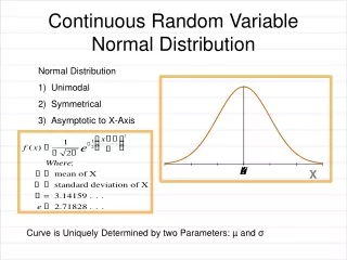
X Continuous Random VariableNormal Distribution • Normal Distribution • Unimodal • Symmetrical • Asymptotic to X-Axis Curve is Uniquely Determined by two Parameters: µ and σ
20 30 40 50 60 70 80 90 100 110 120 Normal Curves for Different Means and Standard Deviations
s = 1 Standardized Normal Distribution • A normal distribution with • a mean of zero, and • a standard deviation of one • Z Formula • standardizes any normal distribution • Z Score • the number of standard deviations which a value is away from the mean
s s = = ? 1 We can find the equivalent point on the Standardized Normal Curve for a point on any other normal Curve. X Z
Z Table • Second Decimal Place in Z • Z 0.00 0.01 0.02 0.03 0.04 0.05 0.06 0.07 0.08 0.09 • 0.00 0.0000 0.0040 0.0080 0.0120 0.0160 0.0199 0.0239 0.0279 0.0319 0.0359 • 0.10 0.0398 0.0438 0.0478 0.0517 0.0557 0.0596 0.0636 0.0675 0.0714 0.0753 • 0.20 0.0793 0.0832 0.0871 0.0910 0.0948 0.0987 0.1026 0.1064 0.1103 0.1141 • 0.30 0.1179 0.1217 0.1255 0.1293 0.1331 0.1368 0.1406 0.1443 0.1480 0.1517 • 0.90 0.3159 0.3186 0.3212 0.3238 0.3264 0.3289 0.3315 0.3340 0.3365 0.3389 • 1.00 0.3413 0.3438 0.3461 0.3485 0.3508 0.3531 0.3554 0.3577 0.3599 0.3621 • 1.10 0.3643 0.3665 0.3686 0.3708 0.3729 0.3749 0.3770 0.3790 0.3810 0.3830 • 1.20 0.3849 0.3869 0.3888 0.3907 0.3925 0.3944 0.3962 0.3980 0.3997 0.4015 • 2.00 0.4772 0.4778 0.4783 0.4788 0.4793 0.4798 0.4803 0.4808 0.4812 0.4817 • 3.00 0.4987 0.4987 0.4987 0.4988 0.4988 0.4989 0.4989 0.4989 0.4990 0.4990 • 3.40 0.4997 0.4997 0.4997 0.4997 0.4997 0.4997 0.4997 0.4997 0.4997 0.4998 • 3.50 0.4998 0.4998 0.4998 0.4998 0.4998 0.4998 0.4998 0.4998 0.4998 0.4998
P( 0 ≤ Z ≤ 1 ) = P( -1 ≤ Z ≤ 1 ) = P( 0 ≤ Z ≤ 2 ) = P( -2 ≤ Z ≤ 2 ) =
P( Z ≥ 1 ) = P( Z ≤ -1.25 ) = P( 1.25 ≤ Z ≤ 2.50) = P( -1.33 ≤ Z ≤ 2.66) = Find C such that Probability is: P( Z ≤ C ) = .80
s = 10 Areas for a Normal Curve with µ = 80 σ = 10 Z P( X ≥ 90 ) = P( X ≤ 65 ) =
P( 65 ≤ X ≤ 90 ) = Find C such that P( X ≥ C ) = .15
Ex 6.45 µ = $951 σ = $96 P( X ≥ $1000 ) = P( 900 ≤ X ≤ 1100 ) =
P( 825 ≤ X ≤ 925 ) = P( X < 700 ) =
Ex 6.12 µ = 200 σ = 47 Find C given this Probability P( X > C ) = .60 P( X < C ) = .83
P( X < C ) = .22 P( X < C ) = .55
Normal Approximation to Binomial Distribution Probabilities Necessary Condition: n ≥ 100 and n•p ≥ 5 We use a Normal Curve which has the same Mean and Std Dev as the Binomial Distribution. Continuity Correction – We will assign all real values for a unit Interval to the single discrete binomial outcome. i.e. X = 40 39.5 ≤ X ≤ 40.5 Ex: 100 Coin Tosses – n = 100 p= .5 q = .5
P100(X=40) ≈ P( 39.5 ≤ X ≤ 40.5) P100(40≤X≤60) ≈ P( 39.5 ≤ X ≤ 60.5)
Ex: 180 Die Rolls – S = 1 Spot n = 180 p = 1/6 q = 5/6 P180(X=25) ≈ P( 24.5 ≤ X ≤ 25.5) P180(X≤25) ≈ P(X ≤ 25.5)
Ex: 6.51 n = 150 p = .75 P150(X < 105) ≈ P150(110≤X≤120) ≈