Download
1 / 17
170 likes | 261 Views
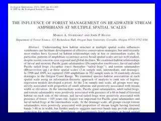
“We sampled amphibians and classified microhabitat in 35 to 50 2-m lengths of stream (sample units) in each drainage (total n 5 702; Fig. 1). We randomly selected five high-, five moderate-, and six low-intensity drainages for study (94-197 ha).

E N D
“We sampled amphibians and classified microhabitat in 35 to 50 2-m lengths of stream (sample units) in each drainage (total n 5 702; Fig. 1). We randomly selected five high-, five moderate-, and six low-intensity drainages for study (94-197 ha).
Quantifying habitat associations at multiple scales Larval Pacific lamprey Benthic sampling (1 m x 1 m). (Torgersen and Close 2004)
Distribution of lamprey larvae among sites Water depth (+) Shade (-) (Torgersen and Close 2004)
Spatial variation within sites Site 29Rkm 9n = 232high density NOT water depth Water velocity (-) % fines in substrate (+)
Spatial scaling and measures of abundance • Spatial binning and smoothing • Measures of abundance (effective density)
Experimenting with bin size… 0 1 km
Spatial smoothing and binning With binning and smoothing… (Torgersen et al. 2008)
What is effective density and why is it important? Standard population density ** Organisms/area sampled = ** Assumes that all habitats within the sampled area are suitable for the organism!
Scaling of abundance measures: Consequences of “binning” Standard pop. density weighted by number of organisms Effective density =
A simple example… 6 m High density 10 m Low density
Effective density and scale of sampling Torgersen et al., unpushed data); Grant et al. 1998. CJFAS. Territory size and the measurement of salmonid abundance. Scaling properties of the organism and its habitat
Grant, J. W. A., S. O. Steingrimsson, E. R. Keeley, and R. A. Cunjak. 1998. Implications of territory size for the measurement and prediction of salmonid abundance in streams. Canadian Journal of Fisheries and Aquatic Sciences 55 (Suppl. 1):181-190. Torgersen, C. E., and D. A. Close. 2004. Influence of habitat heterogeneity on the distribution of larval Pacific lamprey (Lampetra tridentata) at two spatial scales. Freshwater Biology 49:614-630. Torgersen, C. E., R. E. Gresswell, D. S. Bateman, and K. M. Burnett. 2008. Spatial identification of tributary impacts in river networks Pages 159-181 in S. P. Rice, A. G. Roy, and B. L. Rhoads, editors. River confluences, tributaries and the fluvial network. John Wiley & Sons Ltd., Chichester, UK.