Download
1 / 32
320 likes | 333 Views
Understanding the statistical nature of high-energy astrophysics data and its analysis, including the use of statistics to quantify uncertainties and make predictions.

E N D
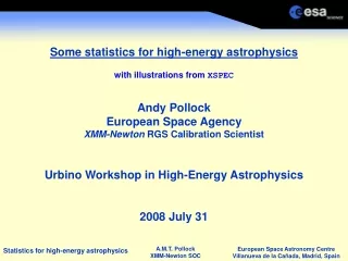
Some statistics for high-energy astrophysics Andy Pollock European Space Agency XMM-Newton RGS Calibration Scientist Urbino Workshop in High-Energy Astrophysics 2008 July 31 with illustrations from XSPEC
Make every photon count. Account for every photon.
Analysis in high-energy astrophysics data models {ni}i=1,N {i}i=1,N 0 individual events continuously distributed detector coordinates physical parameters never change change limited only by physics have no errors subject to fluctuations most precious resource predictions possible kept forever in archives kept forever in journals and textbooks statistics
“There are three sorts of lies: lies, damned lies and statistics.”
Statistical nature of scientific truth • Measurements in high-energy astrophysics collect individual events • Many different things could have happened to give those events • Alternatives are governed by the laws of probability • Direct inversion impossible • Information derived about the universe is not certain • Statistics quantifies the uncertainties : • What do we know ? • How well do we know it ? • Can we avoid mistakes ? • What should we do next ?
There are two sorts of statistical inference • Classical statistical inference • infinite series of identical measurements (Frequentist) • hypothesis testing and rejection • the usual interpretation • Bayesian statistical inference • prior and posterior probabilities • currently popular • Neither especially relevant for astrophysics • one universe • irrelevance of prior probabilities and cost analysis • choice among many models driven by physics
There are two sorts of statistic • 2-statistic • C-statistic • Gaussian statistics • Poisson statistics
There are two sorts of statistics • Gaussian statistics 2 • Poisson statistics C
Gaussian statistics The Normal probability distribution P(x|,) for data={x} and model={,} 1 1/3 2 1/22 3 1/370 4 1/15787 5 1/1744277 1 68.3% 2 95.45% 3 99.730% 4 99.99367% 5 99.999943% P(x|,) -1 +1 x
Poisson statistics The Poisson probability distribution for data={n0} and model={}
Likelihood of data on models {ni}i=1,N data statistics models {i}i=1,N Gaussian Poisson Cash 1979, ApJ, 228, 939
Numerical model of the life of a photon Detected data are governed by the laws of physics. The numerical model should reproduce as completely as possible every process that gives rise to events in the detector: • photon production in the source (or sources) of interest • intervening absorption • effects of the instrument • calibration • background components • cosmic X-ray background • local energetic particles • instrumental noise • model it, don’t subtract it
RGSSAS&CCFcomponents md(coscos BORESIGHT LINCOORDS MISCDATA • rgsproc • atthkgen • rgsoffsetcalc • rgssources • rgsframes • rgsbadpix • rgsevents • evlistcomb • gtimerge • rgsangles • rgsfilter • rgsregions • rgsspectrum • rgsrmfgen • rgsfluxer HKPARMINT ADUCONV BADPIX CROSSPSF CTI LINESPREADFUNC QUANTUMEFF REDIST EFFAREACORR 5-10% accuracy is a common calibration goal
The final data model (,,,D)=S(())R(<>D)+B((D)) D= set of detector coordinates {X,Y,t,PI,…} S =source of interest =set of source parameters R = instrumental response = set of physical coordinates {,,,,…} =set of instrumental calibration parameters B = background =set of background parameters lnL(,,) lnL()
Uses of the log-likelihood, lnL() • lnL is what you need to assess all and any data models • locate the maximum-likelihood model when =* • minimum 2 is a maximum-likelihood Gaussian statistic • minimum C is a maximum-likelihood Poisson statistic • compute a goodness-of-fit statistic • reduced chi-squared 2/ ~ 1 ideally • reduced C C/ ~ 1 ideally • = number of degrees of freedom • estimate model parameters and uncertainties • lnL() • * = {p1,p2,p3,p4,…,pM} • investigate the whole multi-dimensional surface lnL() • compare two or more models • calibrating lnL, 2lnL 2lnL • 2lnL < 1. is not interesting • 2lnL > 10. is worth thinking about (e.g. 2XMM DET_ML 8.) • 2lnL > 100. Hmmm…
Example of a maximum-likelihood solution N-pixel image : data {ni} photons : model {i=spi+b} : PSF pi : unknown parameters {s,b}
Goodness-of-fit • Gaussian model and data are consistent if 2/ ~ 1 • = “number of degrees of freedom” • = number of bins number of free model parameters • = N - M • cf <(x)2/2>=1 • same as comparison with best-possible =0 model, =x, • 2 = 2(lnL(=x)lnL()) • Poisson model and data are consistent if C/ ~ 1 • comparison with best-possible =0 model, =n • 2(nilnnini) 2(nilnii)= 2niln(ni/i)(nii) • XSPEC definition • What happens when many i«1&&ni=0 ? Estimate model parameters and their uncertainties • Parameter error estimates, d, around maximum-likelihood solution, * • 2lnL(*+d) = 2lnL(*) + 1. for 1 (other choices than 1. sometimes made)
Comparison of models • Questions of the type • Is it statistically justified to add another line to my model ? • Which model is better for my data ? • a disk black body with 7 free parameters • a non-thermal synchrotron with 2 free parameters • More parameters generally make it easier to improve the goodness-of-fit • Comparing two models must take into account • {i1} and {i2} • the model with the higher log-likelihood is better • compute 2lnL • 2 > 1,10,100,1000,… (F-test) per extra • C > 1,10,100,1000,… (Wilks’s theorem) per extra • use of probability tables could be required by a referee
Practical considerations • S/ is rarely ~ 1 • S=2|C • lnL(,,) • = set of source spectrum parameters • physics might need improvement • = set of background parameters • background models can be difficult • = set of instrumental calibration parameters • 5 or 10% accuracy is a common calibration goal • solution often dominated by systematic errors • XSPEC’s SYS_ERR is the wrong way to do it • no-one knows the right way (although let’s look at those Gaia people…) • formal probabilities are not to be taken too seriously • S/ > 2 is bad • S/ ~ 1 is good • S/ ~ 0 is also bad • find out where the model isn’t working • pay attention to every bin
The ESA Gaia AGIS idea • Observe 1,000,000,000 stars in the Galaxy • Find the Astrometric Global Iterative Solution • Primary AGIS: For about 10% of all sources (“Primaries”) treat all parameters entering the observational model (S,A,C,G) as unknown. Solve globally as a least-squares minimisation task • Σobservations |observed-calculated(S,A,C,G)|2=min • This yields • Reference attitude, A • Reference calibration, C • Global reference frame, G • Source parameters for 100 million objects, S • Secondary AGIS: Solve for the unknown source parameters of the remaining 900 million sources with least-squares but use A+C+G from previous Primary AGIS solution
Exploration of the likelihood surface lnL() • Frequentists and Bayesians agree that the shape of the entire surface is important • find the global maximum likelihood for = * • identify and understand any local likelihood maxima • calculate 1 intervals to summarise the shape of the surface (time-consuming) • investigate interdependence of source parameters • make lots of plots • why log-log plots ? • Verbunt’s astro-ph/0807.1393 proposed abolition of the magnitude scale • pay attention to the whole model • XSPEC has some relevant methods • XSPEC> fit ! to find the maximum-likelihood solution • XSPEC> plot data ratio ! Is the model good everywhere ? • XSPEC> steppar [one or two parameters] ! go for lunch • XSPEC> error 1. [one or more parameters] ! go home
Gaussian or Poisson ? • The choice you have to make • XSPEC> statistic chisq • XSPEC> statistic cstat • For high counts they are nearly the same (2=n) • (x)2/2 (n)2/n (n)2/ • Gaussian chisq • the wrong answer • the choice of most people • asymptotic properties of 2 goodness-of-fit is probably the reason • rebinning routinely required to avoid low-count bias • n5 or 10 or 25 or 100 according to taste • Poisson cstat • the correct answer for all n0 • my preference • no rebinning necessary • C-statistic also has goodness-of-fit properties
To rebin or not to rebin a spectrum ? • Pros • Gaussian Poisson for n» 0 • dangers of oversampling • saves time • everybody does it • “improves the statistics” • grppha and other tools exist • on log-log plots ln0= • Cons • rebinning throws away information • 0 is a perfectly good measurement • images are never rebinned • Poisson statistics robust for n 0 • 1+2is also a Poisson variable • oversampling harmless • adding bins does not “improve the statistics” Leave spectra alone! Don’t rebin for lnL(). Use Poisson statistics.
Part of the high-resolution X-ray spectrum of Ori XMM RGS Chandra MEG Event count r i f
Error propagation with XSPEC local models • He-like triplet line fluxes • r=resonance, i=intercombination, f=forbidden • Ratios of physical diagnostic significance • R=f/i • G=(i+f)/r • r=norm • i/r=G/(1+R) • f/r= GR/(1+R) • XSPEC> error 1. $G $R SUBROUTINE trifir(ear, ne, param, ifl, photar, photer) INTEGER ne, ifl REAL ear(0:ne), param(8), photar(ne), photer(ne) C--- C XSPEC model subroutine C He-like triplet skewed triangular line profiles C--- C see ADDMOD for parameter descriptions C number of model parameters:8 C 1 WR resonsance line laboratory wavelength (Angstroms) : fixed C 2 WI intercombination line laboratory wavelength (Angstroms) : fixed C 3 WF forbidden line laboratory wavelength (Angstroms) : fixed C 4 BV triplet velocity zero-intensity on the blue side (km/s) C 5 DV triplet velocity shift from laboratory value (km/s) C 6 RV triplet velocity zero-intensity on the red side (km/s) C 7 R f/i intensity ratio C 8 G (i+f)/r intensity ratio
Some general XSPEC advice • Save early and save often • XSPEC> save all $filename1 • XSPEC> save model $filename2 • Beware of local minima • XSPEC> query yes • XSPEC> error 1. $parameterIndex ! go home • Investigate lnL() with liberal use of the commands • XSPEC> steppar [one or two parameters] ! go for lunch • XSPEC> plot contour • Use separate TOTAL and BACKGROUND spectra • Change XSPEC defaults if necessary • Xspec.init • Ctrl^C • Tcl scripting language • Your own local models are often useful • Make lots of plots • XSPEC> setplot rebin …
Example XSPEC steppar results Warning : this took several days - and it’s probably wrong.
XSPEC’s statistical commands • XSPEC12> goodness ! simulation • XSPEC12> bayes ! Bayesian inference • XSPEC12> chain ! Bayesian MCMC methods
General advice • Cherish your data. • Be aware of the strengths and limitations of each instrument. • Don’t subtract from the data, add to the model. • Make lots of plots. • Pay attention to every part of the model. • Think about parameter independence. • 1 errors always. • Same for upper limits. • Make every decision a statistical decision. • Make the best model possible. • If there are 100 sources and 6 different sorts of background in your data, • put 100 sources and 6 different sorts of background in your model. Make every photon count. Account for every photon.