Download
1 / 19
190 likes | 264 Views
Explore how population growth rates can be calculated using various methods like finite, instantaneous, and continuous rates. Learn the formulas and equations to analyze geometric and exponential growth patterns. Understand carrying capacity and the logistic equation in population dynamics.

E N D
Instantaneous and Finite Rates • If interest rate = 10% per year and you start with $100, you will have $110 at the end of the year. 10% is a finite rate. • If interest rate = 5% per half year, you will have $105 after 6 mo. and $110.25 after 1 yr. 5% is a finite rate. • The time interval for calculating interest can be reduced to 0. The interest rate is now an instantaneous rate. • Similarly, rates of population growth can be measured per year, per month, per reproductive season etc. They can also be measured instantaneously.
Converting finite and instantaneous rates • finite rate = einstantaneous ratewhere e = 2.71828 • instantaneous rate = ln finite rate • Let = finite rate; r = instantaneous rate • = er • r = ln • Note: ln is Loge
Geometric Rate of Increase: • Appropriate for species with nonoverlapping generations or for seasonal breeders. • = Nt+1/Nt
l(lambda) • l = Nt+1/Nt • Nt+1 = Ntl
Example of Geometric Growth • = Nt+1/Nt • From below: = 12/6 = 2
Example of Geometric Growth • = Nt+1/Nt • From below: = 12/6 = 2 • Use Nt = N0lt to calculate the population size in 4 years (2005). • N4 = 3(2)4 = 3(16) = 48
Continuous Rates • Nt= N0ert • Appropriate for species with overlapping generations.
Geometric and Exponential Growth • Geometric growth is J-shaped growth described by the equation Nt = N0lt. It increases in increments because reproduction is in increments. • Exponential growth is J-shaped growth described by the equation Nt= N0ert. It increases continuously, producing a smooth curve.
Continuous Growth • At time t, the population size is:Nt= N0ert • At any instant in time, the change in population is:rN
dN dt = rN Change in population size at an instant in time Carrying Capacity Population Size dN dt K-N K = rN Logistic Equation
l(lambda) • N1 = N0l • N2 = N1l • N3 = N2l • N4 = N3l
l(lambda) • N1 = N0l • N2 = N1l • N3 = N2l • N4 = N3l • N257 = ?
l(lambda) • N1 = N0l • N2 = N1l • N3 = N2l • N4 = N3l Notice that N1 is in both of these two equations.
N2 = N0ll = N0l2 l(lambda) • N1 = N0l • N2 = N1l • N3 = N2l • N4 = N3l
l(lambda) • N1 = N0l • N2 = N1l • N3 = N2l • N4 = N3l N2 = N0ll = N0l2 N3 = N0l2l = N0l3
l(lambda) • N1 = N0l • N2 = N1l • N3 = N2l • N4 = N3l N2 = N0ll = N0l2 N3 = N0l2l = N0l3 N4 = N0l3l = N0l4 Nt = N0lt
Finite and Continuous Rates • Finite rate = einstantaneous rate = er • Nt = N0lt replace with er • Nt= N0ert • Appropriate for species with overlapping generations.