Download
1 / 5
50 likes | 73 Views
In this paper, I attempt to pull back the curtains from the Stock Market and figure out how the High Value in the stock market is dependent on the Open Value, Low Value, Close Value. Once that has been done, we will attempt to forecast a model of how the market would act over the next few cycles. We will convert that model into a time series and create the ARIMA model. We will then use the ARIMA model to forecast the possible values for the next cycles. Depending on the forecast values, we will attempt to predict the range of maximum and minimum values. Mitadru Banerjee Chowdhury "Market Index Forecasting Model" Published in International Journal of Trend in Scientific Research and Development (ijtsrd), ISSN: 2456-6470, Volume-4 | Issue-4 , June 2020, URL: https://www.ijtsrd.com/papers/ijtsrd31475.pdf Paper Url :https://www.ijtsrd.com/computer-science/data-processing/31475/market-index-forecasting-model/mitadru-banerjee-chowdhury<br>

E N D
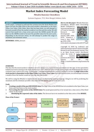
International Journal of Trend in Scientific Research and Development (IJTSRD) Volume 4 Issue 4, June 2020 Available Online: www.ijtsrd.com e-ISSN: 2456 – 6470 Market Index Forecasting Model Mitadru Banerjee Chowdhury Systems Engineer, TCS, West Bengal, Kolkata, India ABSTRACT In this paper, I attempt to pull back the curtains from the Stock Market and figure out how the High Value in the stock market is dependent on the Open Value, Low Value, Close Value. Once that has been done, we will attempt to forecast a model of how the market would act over the next few cycles. We will convert that model into a time series and create the ARIMA model. We will then use the ARIMA model to forecast the possible values for the next cycles. Depending on the forecast values, we will attempt to predict the range of maximum and minimum values. KEYWORDS: ARIMA, forecast How to cite this paper: Mitadru Banerjee Chowdhury "Market Index Forecasting Model" Published in International Journal of Trend in Scientific Research and Development (ijtsrd), ISSN: 2456- 6470, Volume-4 | Issue-4, June 2020, pp.1294-1298, www.ijtsrd.com/papers/ijtsrd31475.pdf Copyright © 2020 by author(s) and International Journal of Trend in Scientific Research and Development Journal. This is an Open Access article distributed under the terms of the Creative Commons Attribution License (CC (http://creativecommons.org/licenses/by /4.0) IJTSRD31475 URL: BY 4.0) OVERVIEW The idea that the stock market is volatile is not new. Rather it is a myth that has percolated over the ages. In fact speculative bubbles have been existing in the stock market since 1637, when the price of Tulip went so high in the Netherlands that when it crashed it sent a nation into a tizzy . In this paper, I attempt to pull back the curtains, and figure out how theHigh Value in the stock market is dependent on the Open Value, Low Value,Close Value.Once that has been done, we will attempt to forecast a model of how the market would act over the next few cycles. We will be using the RStudio to implement the project, in the R programming language. Using R, we will be predicting the maximum and the minimum possible value, that the BSE SENEX can hit in the next cycle. Goals 1. Creating a model of the past BSE SENSEX data:The High Value of the SENSEX has to be modeled on theOpen Value, Low Value and CloeValue on the stock market. 2. Forecasting the time series of the SENSEX data:The model generated has to be turned into a time seriesof the fitted values on the model. 3. Identifying the expected value of the index: Theforecast has to be modeled on the time series of the SENSEX. Flow of the Project @ IJTSRD | Unique Paper ID – IJTSRD31475 | Volume – 4 | Issue – 4 | May-June 2020 Page 1294
International Journal of Trend in Scientific Research and Development (IJTSRD) @ www.ijtsrd.com eISSN: 2456-6470 From the above image of the flow: ?Start:We will install and load all the required packages ?Input: We will be using the BSE historical value in the format of a csv file. ?Processing of Data:This is where we would process the data to see that the formats are matching. ?Creating the Model: We will be using the glmfunction to create a general linear model. We will bemodelling one variable of the data set against the other variables, thus identifying theimpact theindependent variables have on the dependent variable. ?Creating the time series representation of the predicted model: We will be using the ts function, to createthe time series of the fitted valuesof the model. The time series will be modeled on the fitted values of the general linear model. The fitted values represent the values that were predicted which matched with the data set the most. ?Forecasting the time series: We will be forecasting the time series of the fitted values of the model. We willbe forecasting the future by two lags. Technical Flow We need to create a data model for the existing data set as we need to modelthe High Value Against the Low, Close and Open Values.This allows us to understand the impact the Low,Close and Open Values are having on High Value. The Model will find the relationship between the High Values and other variables. This relation can be modeled using either +, * or: . ?By using the ‘:’, we will find the relationship between the interaction terms of the variables. ?By using the ‘*’, we will include both the variables and the interaction term. ?By using the ‘+’, we will include only the impact the variables have on each other and not their interaction terms. We will then be comparingthe models based on their AIC scores.The model would help us identify the impact the Open, Close and Low price has on the High price. We need to compare the models created and pick the one which has the least value of AIC, as it would mean that this would have the least variance. This would allow us to create a time series for the fitted values (The values that would actually match the data set) of that model. Lower the value of AIC, better is the model. AIC is one way to understand which model best represents the set of data. Then we would be able to createthe time series component of the Fitted values (This is essentially the High Values of the Model) of the model. The time series would represent the change in the fitted values of the model over time. We would have to stabilize the time series by diffingthe time series.The next step would be to create an ARIMA model,to create a model of the time series with the lags of itself. Then we will be comparing the residuals of the models, to see if they are whitenoiseor not. That would help prove the efficacy of the model. If the residual corresponds to white noise, then we can be sure that the model is good. Packages ?ggplot2: To plot the model. ?Forecast: To forecast the time series of the data set. ?Scales: Used to dress the data set. Steps 1.Loading the packages required for the project: To install the packages required for the project, we will follow the following steps: Install.packages (“ggplot2”) Install.packages (“forecast”) Install.packages (“scales”) 2.Processing the Inputs: To process the model, we will be using the BSE SENSEX index over the last 10 years. We can find the historical value of the SENSEX from the website: (https://www.bseindia.com/Indices/IndexArchiveData.html). The data set can be downloaded in the form of a csv file. You can find the csv file used for this project here: You can read the file as a data set by the following command: BSESensex<-read.csv (file.choose()) [#Youcan then choose the file which was downloaded] @ IJTSRD | Unique Paper ID – IJTSRD31475 | Volume – 4 | Issue – 4 | May-June 2020 Page 1295
International Journal of Trend in Scientific Research and Development (IJTSRD) @ www.ijtsrd.com eISSN: 2456-6470 Plot of the High Price of the BSE SENSEX Index from 2010-2020. We can plot the above graph by the following code: plot(BSESensex$High,type = "h",col=BSESensex$Date,main = "The plot of the High values over time in BSE SENSEX from 2010- 2020",xlab = "Time passage in days",ylab = "Index Price") We can plot the High Values of the Data Set, over time, as stepwise growth. We can plot the above graph, by the following code: plot(BSESensex$High,type = "S",main="Plot of the High Value of the BSE Sensex index",xlab = "Time",ylab = "BSE SENSEX Index Value") 3.Data Pre-processing This is a vital step, as it will help us both shape the data. The data that has been downloaded from the BSE website, has the dates arranged in a non csv format. We have to save the Data in the csv format, for us to process the data easily. 4.Data Model To create the data model, we have to consider that the Highvalueis dependent on three factors, OpenPrice, Close Priceand Low PriceWe create a general linear model of the High value as dependent on theOpen and Low values. BSEModel<-glm(BSE$High~BSE$Open*BSE$Low*BSE$Close) @ IJTSRD | Unique Paper ID – IJTSRD31475 | Volume – 4 | Issue – 4 | May-June 2020 Page 1296
International Journal of Trend in Scientific Research and Development (IJTSRD) @ www.ijtsrd.com eISSN: 2456-6470 This creates the general linear model, BSEModel, which will have the fitted values and the residuals. The BSEModel$fitted.values, represent the values which are the best fit. The BSEModel$residuals represent the values that have not been fitted into the model. The following code can be implemented to create the model. The code to create and test the Models created: BSESensexModel1<-glm(BSESensex$High~BSESensex$Open*BSESensex$Low*BSESensex$Close) BSESensexModel2<-glm(BSESensex$High~BSESensex$Open+BSESensex$Low+BSESensex$Close) BSESensexModel3<-glm(BSESensex$High~BSESensex$Open*BSESensex$Low+BSESensex$Close) BSESensexModel4<-glm(BSESensex$High~BSESensex$Open+BSESensex$Low*BSESensex$Close) BSESensexModel5<-glm(BSESensex$High~BSESensex$Open:BSESensex$Low:BSESensex$Close) BSESensexModel6<-glm(BSESensex$High~BSESensex$Open:BSESensex$Low+BSESensex$Close) BSESensexModel7<-glm(BSESensex$High~BSESensex$Open:BSESensex$Low*BSESensex$Close) BSESensexModel8<-glm(BSESensex$High~BSESensex$Open:BSESensex$Low+BSESensex$Close) BSESensexModel9<-glm(BSESensex$High~BSESensex$Open+BSESensex$Low:BSESensex$Close) BSESensexModel10<-glm(BSESensex$High~BSESensex$Open*BSESensex$Low:BSESensex$Close) AIC(BSESensexModel1,BSESensexModel2,BSESensexModel3,BSESensexModel4,BSESensexModel5,B SESensexModel6,BSESensexModel7,BSESensexModel8,BSESensexModel9,BSESensexModel10) Plot of the Fitted Values of BSE SENSEX Model plot(BSESensexModel2$fitted.values,type="h",main="Plot of the Fitted Values of the BSE Sensex model.",xlab="Time in years",ylab="BSE SENSEX Index value",col=BSESensexModel2$coefficients) 5.Time Series of the fitted values We will convert the fitted values of the Model into a time series. We will then plot the Time Series, to chart the trend line of the values. BSEFittedTS holds the time series of the fitted values of the model. Plot of the Time Series representation of the Fitted Values of Sensex Model. @ IJTSRD | Unique Paper ID – IJTSRD31475 | Volume – 4 | Issue – 4 | May-June 2020 Page 1297
International Journal of Trend in Scientific Research and Development (IJTSRD) @ www.ijtsrd.com eISSN: 2456-6470 plot(BSESenseTimeSeries,main="Plot of the Time Series representation of the Fitted Values of the Sensex model.",xlab="Time in years",ylab="BSE SENSEX Index value") 6.ARIMA and Forecasting the Time Series We will create an ARIMAModelof the time series, to create an auto-regressiveand movingaveragemodel of the Time Series. We will use this model to forecast the possible values of the time series.The idea is to predict the possible range of values for a cycle in the future. Code to create the Arima Model of the BSESensex Time Series: #Calculating the ARIMA model of the Time Series BSESensexArimaModel<-auto.arima(BSESensexTimeSeries) #Calculating the Forecast of the BSESensexArimaModel, fitted values. BSESensexArimaForecast<-forecast(BSESensexArimaModel$fitted)plot(BSESensexArimaModel$fitted) Plot of BSE SENSEX Forecast against the year plot(BSESensexArimaForecast,type = "h",main = "Plot of BSE SENSEX Forecast against the years",xlab = "Time in years",ylab = "Index value of BSE Sensex",col = BSESensexArimaForecast$x) It is vital to figure out the maximum and minimum possible values for the next cycle. We will be finding the maximum and minimum possible values, from the forecast Data Frame. We will be using the BSESensexArimaForecast, to understand the approximate movement of the Index. > max(BSESensexArimaForecast$fitted) [1] 42143.86 > min(BSESensexArimaForecast$fitted) [1] 15370.33 Conclusion In the project we: ?Loaded the data. ?Created multiple models. ?Compared the models, to find out the best fit. ?Created a time series of the fitted values of the model. ?Created the ARIMA model of the time series. ?Forecast the model. ?Plot the forecast. ?Predict the range of possible values for the next cycle. Thus we predicted the values of the model. All resources of the project can be found in the provided link. @ IJTSRD | Unique Paper ID – IJTSRD31475 | Volume – 4 | Issue – 4 | May-June 2020 Page 1298