Download
1 / 29
290 likes | 353 Views
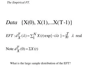
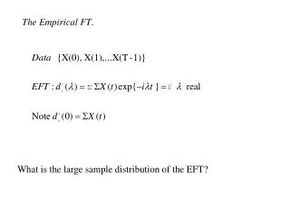
The Empirical FT. What is the large sample distribution of the EFT?. The complex normal. Theorem. Suppose X is stationary mixing, then. Proof. Write. Evaluate first and second-order cumulants Bound higher cumulants Normal is determined by its moments. Consider. Comments .

E N D
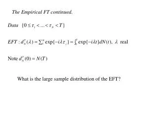
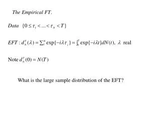
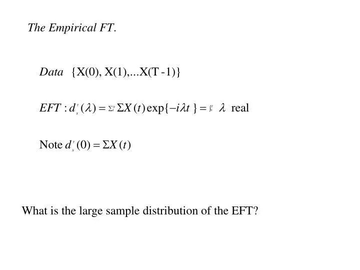
The Empirical FT. What is the large sample distribution of the EFT?
Proof. Write Evaluate first and second-order cumulants Bound higher cumulants Normal is determined by its moments
Comments. Already used to study rate estimate Tapering makes Get asymp independence for different frequencies The frequencies 2r/T are special, e.g. T(2r/T)=0, r 0 Also get asymp independence if consider separate stretches p-vector version involves p by p spectral density matrix fXX( )
Estimation of the (power) spectrum. An estimate whose limit is a random variable
Some moments. The estimate is asymptotically unbiased Final term drops out if = 2r/T 0 Best to correct for mean, work with
Periodogram values are asymptotically independent since dT values are - independent exponentials Use to form estimates
Estimation of finite dimensional . approximate likelihood (assuming IT values independent exponentials)
Crossperiodogram. Smoothed periodogram.
Large sample distributions. var log|AT| [|R|-2 -1]/L var argAT [|R|-2 -1]/L
Advantages of frequency domain approach. techniques formany stationary processes look the same approximate i.i.d sample values assessing models (character of departure) time varying variant ...
Networks. partial spectra - trivariate (M,N,O) Remove linear time invariant effect of M from N and O and examine coherency of residuals,
Point process system. An operation carrying a point process, M, into another, N N = S[M] S = {input,mapping, output} Pr{dN(t)=1|M} = { + a(t-u)dM(u)}dt System identification: determining the charcteristics of a system from inputs and corresponding outputs {M(t),N(t);0 t<T} Like regression vs. bivariate
Realizable case. a(u) = 0 u<0 A() is of special form e.g. N(t) = M(t-) arg A( ) = -