Download
1 / 19
240 likes | 421 Views
6 th Annual GIScience in Higher Education Summit March 21, 2014 — University of Denver. Precision Agriculture: A Transformative Teaching Moment for Geotechnology.

E N D
6th Annual GIScience in Higher Education Summit March 21, 2014 — University of Denver Precision Agriculture:A Transformative Teaching Moment for Geotechnology To many, Precision Agriculture seems like an oxymoron. With mud up to the axles and 400 acres left to plough, precision seems worlds away. Yet site-specific management makes sense to a rapidly growing number of farmers. Mapping and analyzing variability in field conditions, and linking such spatial relationships to management action, places production agriculture at the cutting edge of GIS applications. …all this from an industry that just two decades ago only used maps for hunting elk …this presentation investigates the use of Precision Ag’s unique expression of Geotechnology as an effective vehicle for teaching fundamental GIS concepts and procedures Presentation by Joseph K. Berry Adjunct Faculty, Department of Geography, University of Denver Adjunct Faculty, Warner College of Natural Resources, Colorado State University Principal, Berry & Associates // Spatial Information Systems Email jberry@innovativegis.com — Website www.innovativegis.com/basis/ (See http://www.innovativegis.com/basis/present/GISinHigherEd2014/to access support materials including this PowerPoint)
Some Examples ofSoaring PA Technology Applications 1) LiDAR Imaging vs. RTK GPS (terrain surface) LiDARfor regional/state-wide surveys RTK GPSfor farm-level survey LiDAR andRTKfor multistage terrain analysis RTK GPS LiDAR Tom Buman’s Precision Conservation blog at http://precisionconservation.com/ 2) Automated 3D Machines (controlling positioning/hydraulics) Field Grading to level a field Optimal Field Tileplacement Variable-rate Seeding(depressions) Laser Leveling Eyeball Leveling http://www.fao.org/docrep/t0231e/t0231e08.htm/ 3) Remote Sensing Imagery andDrone Technology Remote Sensing: Satellite and Hyperspectral Imagingfor crop development Drones: Geometric registration for Farm/Compliance Mapping Spectral analysis for Field Scouting Possibly for Spot Spraying (Future) http://www.specterra.com.au/precision_agriculture.html http://aerialfarmer.blogspot.com/ (Berry)
More Examples ofSoaring PA Technology Applications 4) Ground Instrumentation for weather, soil moisture, harvesting Farm-based Weather Stationsfor disease, insect and water monitoring In-field network of Soil Moisture Probesfor Evapotranspiration (ET) modeling Robotic Machinesthat can operate autonomously Advances in Crop Yield Monitor accuracy Advances in Field Samplingand Map Surface Generation Yield Monitor Mass Flow = time for material to move from the harvest point to the yield monitor GPS Interpolation Error “Trolling for Yield Data” 5) New Technology Environment Faster/Cheaper/Smaller computers/tablets/phones Ubiquitous Connectivity from farm base to field to cafe Cloud Computingcapabilities (more available and accessible) Physical Distance (1sec at 4mph = 5.86ft) 6) Evolving Legal, Regulatory, Business and Social Environments As Applied Mapping for regulatory compliance and organic/GMO certification Data Ownership, Convertibility and Sharing will become increasingly important Integrated Platform Solutions from a few large companies will replace the disparate pieces of a solution from various small companies Scale, Expense and Cyber-phobia will continue as entry constraints but diminish as the farm community becomes more comfortable with computer technology (Berry)
Yield Limiting Factors (the basis of PA) • Water • Weather • Topography • Nutrients • Weeds • Pests • Genetics • Seeding Rate • Other… • Candidate factorfor Precision Agriculture and Site-specific Management • if and only if — • the factor is a significant driving variable • it has measurable spatial variability • its spatial variation can be explained and spatial relationships established • it exhibits a spatial response to practical management actions …and results in production gains, increased profitability and/or improved stewardship (Berry)
Whole-fieldassumes the “average” conditions are the same everywhere within the field(uniform/homogenous) Management action is the same throughout the field Discrete Management Zones break the field into areas of similar conditions(zones) Management action is the same within each zone …manage as a set of small irregular sub-fields Z2 Continuous Map Surfaces break the field into small consistent pieces (grid cells) that track specific conditions at each grid location Z1 Z1 Z3 Management action varies continuously throughout the field Z2 Whole Fieldvs.Site Specific Management Aggregated Space Aggregated Space The bulk of agricultural research has been “non-spatial” (Spatially Aggregated) …but PA is all about disaggregated spatial relationships/patterns— Research Opportunity Disaggregated Space (Berry)
Data Analysis Perspectives (Data Space vs. Geographic Space) Map Analysis (Geographic Space — Spatial Statistics) Interpolated Surface fit to the data (density function) Average = 22.0 StDev = 18.7 Typical How Typical 22.0 28.2 Identifies the Typical Value Maps the Variance Traditional Analysis (Data Space — Non-spatial Statistics) Standard Normal Curve fit to the data (density function) Field Data Histogram Point Data Plot Central Tendency Continuous Spatial Distribution (Detailed) “Thousands of Values” Discrete Spatial Object (Generalized) “Single Value” (Berry)
Grid-based Map Analysis Approaches Map Analysis involves three broad types of “Analytical Tools”— Interpolated Surface (Phosphorous Layer) • Surface Modelingmaps the spatial distributionof point-sampled data • Map Generalization— characterizes spatial trends (e.g., tilted plane) • Spatial Interpolation— continuous spatial distribution (e.g., IDW, Krig) • Other— roving windows and facets (e.g., density surface, tessellation) • Surface Modelingmaps the spatial distribution of point-sampled data • Map Generalization— characterizes spatial trends (e.g., tilted plane) • Spatial Interpolation— continuous spatial distribution (e.g., IDW, Krig) • Other— roving windows and facets (e.g., density surface, tessellation) Point Samples (P,K,N) • Spatial Statisticsinvestigates the “numerical” relationships in mapped data • Descriptive— aggregate statistics (e.g., average, stdev, similarity, clustering) • Predictive— relationships among map layers (e.g., regression) • Prescription— appropriate actions (e.g., decision rules, optimization) Geo-registered Map Layers (P,K,N) Data Clusters (P,K,N) • Spatial Analysisinvestigates the “contextual” relationships in mapped data • Reclassify— reassigns map values (e.g., position, value, shape, contiguity) • Overlay— map layer coincidence (e.g., point-by-point, region-wide, map-wide) • Distance— proximity and connection (e.g., movement, optimal paths, visibility) • Neighbors— roving windows (e.g., slope, aspect, diversity, anomaly) Erosion Potential fn(Slope, Flow) Field Elevation (Berry)
Corn Field Phosphorous (P) Data “Spikes” IDW Surface Spatial Interpolation (soil nutrient levels) Spatial Interpolationmaps the geographic distributioninherent in data sets (Berry)
Comparison of the IDW interpolated surface to the whole field Average shows large differences in localized estimates (-16.6 to 80.4 ppm) Comparison of the IDW interpolated surface to the Krig interpolated surface shows small differences in localized estimates (-13.3 to 11.7 ppm) Comparing Spatial Interpolation Results (Berry)
Grid-based Map Analysis Approaches Map Analysis involves three broad types of “Analytical Tools”— Interpolated Surface (Phosphorous Layer) • Surface Modelingmaps the spatial distribution of point-sampled data • Map Generalization— characterizes spatial trends (e.g., tilted plane) • Spatial Interpolation— derives a continuous spatial distribution (e.g., IDW, Krig) • Other— roving windows and facets (e.g., density surface, tessellation) Point Samples (P,K,N) • Spatial Statisticsinvestigates the “numerical” relationships in mapped data • Descriptive— aggregate statistics (e.g., average, stdev, similarity, clustering) • Predictive— relationships among map layers (e.g., regression) • Prescription— appropriate actions (e.g., decision rules, optimization) • Spatial Statisticsinvestigates the “numerical” relationships in mapped data • Descriptive— aggregate statistics (e.g., average, stdev, similarity, clustering) • Predictive— relationships among map layers (e.g., regression) • Prescription— appropriate actions (e.g., decision rules, optimization) Geo-registered Map Layers (P,K,N) Data Clusters (P,K,N) • Spatial Analysisinvestigates the “contextual” relationships in mapped data • Reclassify— reassigns map values (e.g., position, value, shape, contiguity) • Overlay— map layer coincidence (e.g., point-by-point, region-wide, map-wide) • Distance— proximity and connection (e.g., movement, optimal paths, visibility) • Neighbors— roving windows (e.g., slope, aspect, diversity, anomaly) Erosion Potential fn(Slope, Flow) Field Elevation (Berry)
Interpolated Spatial Distribution Phosphorous (P) What spatial relationships do you see? Visualizing Spatial Relationships …do relatively high levels of P often occur with high levels of K and N? …how often? …where? Humans can only “see” broad Generalized Patterns in a single map variable… (Berry)
Clustering Maps for Data Zones …but computers can “see” detailed patternsin multiple map variables (using Data Space) Geographic Space …groups of “floating balls” in data space identify locations in the field with similar data patterns–Data Zones(Data Clusters) …or a Continuous Equation precisely identifying the right action for each grid cell (Berry)
The Precision Ag Process(Fertility example) …there are four fundamental steps in the Precision Ag Process— Dependent Map Variable Prescription Map Zone 3 Yield Map On-the-Fly “Intelligent Implements” Nutrient Maps Derived Zone 2 Zone 1 Variable Rate Application Independent Map Variables 1) Data Collection 4) Management Action 2) Data Analysis 3) Modeling …the process is more generally termed Spatial Data Miningand is used in a host of applications from Geo-business to Epidemiology to Infrastructure Routing to Wildfire Risk Modeling …etc. and is analogous to non-spatial “Quantitative Data Analysis”— but uses “Map Variables” (Berry)
Grid-based Map Analysis Approaches Map Analysis involves three broad types of “Analytical Tools”— Interpolated Surface (Phosphorous Layer) • Surface Modelingmaps the spatial distribution of point-sampled data • Map Generalization— characterizes spatial trends (e.g., tilted plane) • Spatial Interpolation— derives a continuous spatial distribution (e.g., IDW, Krig) • Other— roving windows and facets (e.g., density surface, tessellation) Point Samples (P,K,N) • Spatial Statisticsinvestigates the “numerical” relationships in mapped data • Descriptive— aggregate statistics (e.g., average, stdev, similarity, clustering) • Predictive— relationships among map layers (e.g., regression) • Prescription— appropriate actions (e.g., decision rules, optimization) Geo-registered Map Layers (P,K,N) Data Clusters (P,K,N) • Spatial Analysisinvestigates the “contextual” relationships in mapped data • Reclassify— reassigns map values (e.g., position, value, shape, contiguity) • Overlay— map layer coincidence (e.g., point-by-point, region-wide, map-wide) • Distance— proximity and connection (e.g., movement, optimal paths, visibility) • Neighbors— roving windows (e.g., slope, aspect, diversity, anomaly) • Spatial Analysisinvestigates the “contextual” relationships in mapped data • Reclassify— reassigns map values (e.g., position, value, shape, contiguity) • Overlay— map layer coincidence (e.g., point-by-point, region-wide, map-wide) • Distance— proximity and connection (e.g., movement, optimal paths, visibility) • Neighbors— roving windows (e.g., slope, aspect, diversity, anomaly) Erosion Potential fn(Slope, Flow) Field Elevation (Berry)
Micro Terrain Analysis(a simple field erosion/pooling model) times 10 plus renumber Field Elevationis formed by assigning an elevation value to each cell in an analysis grid (1cm Lidar) Determining Erosion/PoolingPotential: Slopeclasses (1= Gentle, 2=Moderate, 3= Steep) and Flowclasses (1= Light, 2=Moderate, 3= Heavy Flows) …are combined into a single map identifying erosion/pooling potential 33= Steep & Heavy 1= Gentle 2= Mod 3= Steep 11= Gentle & Light 1= Light 2= Mod 3= Heavy …map of the Effective Movement (surface flow) of water, fine particles and organic matter within a field (Berry)
Precision Conservation(compared to Precision Ag) Wind Erosion Chemicals SoilErosion Runoff Leaching 3-Dimensional Movements Precision Conservation Precision Ag …closely related disciplines Terrain 2-Dimensional Data Layers Soils 2D Square 3D Cube Yield Potassium Coincidence Landscape Perspective Field Perspective CIR Image (Ecological emphasis) (Production Emphasis) Landscape Field Precision Conservationconnects farm fields, grasslands, rangelands and managed forests with their natural surrounding areas such as buffers, riparian zones, natural forest, and water bodies... then uses information about localized surface and subsurface flows and cycles to analyze and better understand ecosystem processes leading to the best management practices for conservation and sustainability of agricultural, rangeland, and natural areas. (Berry)
Calculating Effective Distance(variable-width buffers) Effective erosion buffersaround a stream expand and contract depending on the erosion potential of the intervening terrain Reach out farther under high Erosion Potential (Berry)
Water Conservation Modeling (Conservation = “wise use”) US Drought Monitor West Water Rights Historic Crop Water Allocation Alternative Water Budget Crop Water Allocation Crops City Purchase all rights …and move to the city Farm Income City Water Farm “Win-Win-Win” “Buy andDry” To River To River Temporary Monitored Transfers Farmland Farmland Grid-based Map Analysis/Modelingof consumptive water needs and optimization to increase farm revenue based on New/Expanded Instrumentation: Water Flow Measurements — Irradiation/Evapotranspiration Monitoring — Soil Moisture Measurements — Remote Sensing Sustainable Water and Innovative Irrigation Management (SWIIM) http://www.regenmg.com/Home.aspx (Berry)
Where To Go From Here… www.innovativegis.com/basis/ Present/PAConf_Calgary2014/ Online References Plenary Session (1.25hr; 27 fully annotated slides) Precision Agriculture’s Bold New Era …a brief history, current expression and radical new directions Breakout Session (1.00hr; 16 fully annotated slides) Returning the Scientific Horse to in Front of the Technical Cart …a math/stat framework for Map Analysis Beyond Mapping Compilation Series …Beyond Mapping columns appearing in GeoWorld magazine from March 1989 through December 2013 organized into four downloadable books Presentation handout (Berry)