Download
1 / 28
280 likes | 447 Views
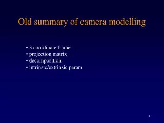
Old summary of camera modelling. 3 coordinate frame projection matrix decomposition intrinsic/extrinsic param. World coordinate frame: extrinsic parameters. Finally, we should count properly . ‘new’ way of looking at ‘old’ modeling. ‘abstract’ camera: projection from P3 to P2.

E N D
Old summary of camera modelling • 3 coordinate frame • projection matrix • decomposition • intrinsic/extrinsic param
World coordinate frame: extrinsic parameters Finally, we should count properly ...
‘new’ way of looking at ‘old’ modeling ‘abstract’ camera: projection from P3 to P2 Math: central proj. Physics: pin-hole As lines are preserved so that it is a linear transformation and can be represented by a 3*4 matrix This is the most general camera model without considering optical distortion
Properties of the 3*4 matrix P • 11 d.o.f. • Rank(P) = ? • ker(P)=c • row vectors, planes • column vectors, directions • principal plane: w=0 • calibration, 6 pts • decomposition by QR, • K intrinsic (5). R, t, extrinsic (6) • geometric interpretation of K, R, t (backward from u/x=v/y=f/z to P) • internal parameters and absolute conic
What is the calibration matrix K? It is the image of the absolute conic, prove it first! Point conic: The dual conic:
Don’t forget: when the world is planar … A general plane homography!
Camera calibration Given from image processing or by hand • Estimate C • decompose C into intrinsic/extrinsic
Calibration set-up: 3D calibration object
The remaining pb is how to solve this ‘trivial’ system of equations!
Review of some basic numerical algorithms • linear algebra: how to solve Ax=b? • (non-linear optimisation) • (statistics)
Linear algebra review • Gaussian elimination • LU decomposition • orthogonal decomposition • QR (Gram-Schmidt) • SVD (the high(est)light of linear algebra!)
Solving (full rank) square matrix linear sys Ax =b = elimination = LU factorization • factor A into LU • solve Lc = b (lower triangular, forward substitution) • solve Ux=c (upper tri., backward substitution)
Solving for Least squares solution for Ax=b, min||Ax-b|| = pseudo-inverse x = (A^TA)-1(A^T A)b (theoretically, but not numerically) Orthogonal bases and Gram-Schmidt A = QR Numerically, QR does it well: as A^TA= R^TR,
Solving for homogeneous system Ax=o subject to ||x||=1, It is equivalent to min||Ax||, i.e. x^T A^T A x, the solution is the eigenvector of A^TA associated with the smallest eigenvalue Triangular systems not bad, but diagonal system is better! Diagonalization = eigen vectors => doable for symmtric matrices
row space: first Vs • null space: last Vs • col space: first Us • null space of the trans : last Us SVD gives orthogonal bases for all subspaces You get everything with svd: A x = b, pseudo-inverse, x = A+ b for both square system and least squares sol. Even better with homogeneous sys: A x =0, x = v_n !
Linear methods of computing P • p34=1 • ||p||=1 • ||p3||=1 Geometric interpretation of these constraints
Decomposition • analytical by equating K(R,t)=P • (QR (more exactly it is RQ))
Renormalise by c3 • tz = c34 • r3 = c3 • u0 = c1^T c3 • v0 = c2^T c3 • alpha u • alpha v • …
Linear, but non-optimal,but we want optima, but non-linear, methods of computing P
(Non-linear iterative optimisation) • J d = r from vector F(x+d)=F(x)+J d • minimize the square of y-F(x+d)=y-F(x)-J d = r – J d • normal equation is J^T J d = J^T r (Gauss-Newton) • (H+lambda I) d = J^T r (LM) Note: F is a vector of functions, i.e. min f=(y-F)^T(y-F)
Using a planar pattern Why? it is more convenient to have a planar calibration pattern than a 3D calibration object, so it’s very popular now for amateurs. Cf. the paper by Zhengyou Zhang (ICCV99), Sturm and Maybank (CVPR99) (Homework: read these papers.)
first estimate the plane homogrphies Hi from u and x, • 1. How to estimate H? • 2. Why one may not be sufficient? • extract parameters from the plane homographies
How to extract intrinsic parameters? Relationship between H and parameters:
(How to extract intrinsic parameters?) The absolute conic in image The (transformed) absolute conic in the plane: The circular points of the Euclidean plane (i,1,0) and (-i,1,0) go thru this conic: two equations on K!
What does the calibration give us? It turns the camera into an spherical one, or angular/direction sensor! Normalised coordinates: Direction vector: Angle between two rays ...
Summary of calibration • Get image-space points • Solve the linear system • Optimal sol. by non-linear method • Decomposition by RQ