Download
1 / 7
70 likes | 346 Views
On A Laboratory, “Magnetic Resonance” Experimental Set up. This is an Animated feature Viewable ONLY with the MS PowerPoint XP Version. Other versions would not enable all the animation Features Effectively.

E N D
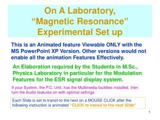
On A Laboratory, “Magnetic Resonance” Experimental Set up This is an Animated feature Viewable ONLY with the MS PowerPoint XP Version. Other versions would not enable all the animation Features Effectively. An Elaboration required by the Students in M.Sc., Physics Laboratory in particular for the Modulation Features for the ESR signal display system. If your System, the P.C. Unit, has the Multimedia facilities installed, then turn the Audio features on with optimal settings Each Slide is set to transit to the next on a MOUSE CLICK after the following instruction is animated“CLICK to transit to the next Slide”
A Thumb rule to work out Electron Spin Resonance Frequency is as follows: since hν=gβH is the relation governing resonance condition, by knowing the relevant constants from available data tables, it should be verified that the following equation closely approximates the resonance frequency-field criterion for ESR. 1 Gauss = 2.8 MHz for a free electron spin with g=2 Therefore if one can detect the oscillator levels using an oscillator-detector, and , if the frequencies of the oscillations are in the range of 8-32 MHz, then using the above equation the corresponding resonance field can be calculated. 2.9 – 11.5 Gauss. Further a simple Helmholtz coil can be designed to obtain these Magnetic Field Strengths by providing a suitably designed current sources which may be available even commercially. Then a Block Diagram of the type shown in the next slide can be appropriate for constructing and assembling a esr detection system. CLICK to transit to next slide
Oscillation Level reduced when there is ESR absorption Oscillation Level at fixed frequency ‘ν’ When No ESR Detected DC Level No ESR 2 Oscillator Oscillation Level Detector 1 ΦShifter Reduced DC On ESR Absorption hν=gβH Detected Oscln Level DC No oscillations 0 The role of a phase Φshifter in the diagram would be explained in the succeeding slides If the Current is increased from 0 to beyond resonance field, then, the field [ Ht] increases with time and causes resonance at resonance field value Ht hν=gβH 2 1 Current Source CLICK to transit to next slide
Click to transit to next slide Since the Magnetic Field values are in the range of 10 gauss only instead of a steadily increasing field a sinusoidal field variation with time can be generated and the magnetic field can be swinging back and forth about zero field value and the peak value of this sinusoidal field variation can be larger than the resonance field value. Thus from zero while swinging positive the resonance can occur, next when from the peak positive value when the field swings towards zero once more there will be resonance. Since ESR resonance condition can be valid without any regard to field directions but depending only on the magnitude, there can be twice resonance during the negative swing. Thus the Resonance Condition is better expressed by h ν = g β |H| This sinusoidal variation has the time dependence as below: H t = H psin ( 2πf t + φ ) Ht is the instantaneous value of the Field and Hp is the peak value during the sinusoidal variation of the field with time. Φis the phase of this variation. f is the frequency of the variation which is significantly small only of the order of few tens Hertz while the ESR resonance frequency would be in the Megahertz range. This field variation is caused by an electrical current and this electrical signal can be applied to the X axis of an oscilloscope display while the Y axis would be the detected RF signal – a DC, in the absence of the time varying magnetic field. In this process there can be phase differences in the sinusoidal variation of the Magnetic Field and the X axis trace of the oscilloscope and it would be necessary to introduce a phase shifter in the circuit.
hν = gβH resonace condition encountered twice: 1st at +H : 2nd at -H Click & transit to next Slide In Phase Modulation Peak to Peak modulation amplitude =2Hp -HP to +HP +H 1 Oscilloscope display trace 0 Cursor arrow position indicates H t 2 -H X input Current on Sinusoidal Field Variation with Center zero
hν = gβH resonace condition encountered twice: 1st at +H : 2nd at -H CLICK to transit to the Last slide of this slide show a Out of Phase Modulation 2 +H b Oscilloscope display trace 0 -H a 1 b X input Current on Sinusoidal Field Variation with Center zero
An Assignment • The illustration till now demonstrated the consequence of a 90º phase shift between the sinusoidal modulation of the Field and the Input to the X axis of Oscilloscope. Obviously the field variations can be described with a Sine function where as in the second setting the X axis input was Cosine function. • Try to make a similar Animated feature for phase difference of 10º, 45º, and 60º and view the resulting sequence in which the several resonance coincidences occur and visualize what the oscilloscope display would be for a modulation frequency of about 60Hz. CLICK to transit to the First Slide