Download
1 / 68
810 likes | 1.15k Views
Introduction to Simulink. Dr. Mohammed F. Alsayed. Introduction. In the last few years, Simulink has become the most widely used software package in academia and industry for modeling and simulating dynamical systems .

E N D
Introduction to Simulink Dr. Mohammed F. Alsayed
Introduction • In the last few years, Simulink has become the most widely used software package in academia and industry for modelingand simulatingdynamical systems. • Simulinkenvironment encourages you to pose a question, model it, and see what happens. • You can move beyond idealized linear models to explore more realistic nonlinear models. Thus, describing real-world phenomena. • It turns your computer into a lab for modeling and analyzing systems.
What is Simulink? • It is a software package for modeling, simulating, and analyzing dynamical systems. • It supports linear and nonlinear systems, modeled in continuous time, sampled time, or a hybrid of the two. • Systems can also be multirate, i.e., have different parts that are sampled or updated at different rates.
What is Simulink? • For modeling, Simulink provides a graphical user interface (GUI) for building modelsas block diagrams, using click-and-drag mouse operations. • With this interface, you can draw the models just as you would with pencil and paper. • You can also customize and create your own blocks (S-Functions). • Models are hierarchical, so you can build models using both top-downand bottom-upapproaches.
What is Simulink? • After you define a model, you can simulate it, using a choice of integration methods, either from the Simulink menus or by entering commands in MATLAB’s command window. • You can change parameters and immediately see what happens, for “what if” exploration. • The simulation results can be put in the MATLABworkspace for postprocessingand visualization
Quick Start Running a Demo model • An interesting demo program provided with Simulink models the thermodynamics of a house. • To run this demo, type thermo in the MATLAB command window. This command starts up Simulink and creates a model window that contains this model. or >> demo ‘simulink’
Quick Start • When you open the model, Simulink opens a Scope block containing two plots labeled Indoor vs. Outdoor Temp and Heat Cost ($), respectively. • To start the simulation, pull down the Simulation menu and choose the Startcommand (or, on Microsoft Windows, press the Start button on the Simulinktoolbar). • As the simulation runs, the indoor and outdoor temperatures appear in the Indoor vs. Outdoor Temp plot and the cumulative heating cost appears in the Heat Cost ($) plot.
Quick Start • To stop the simulation, choose the Stop command from the Simulation menu (or press the Pause button on the toolbar). • When you’re finished running the simulation, close the model by choosing Close from the File menu.
Quick Start Description of the Demo • The demo models the thermodynamics of a house using a simple model. The thermostat is set to 70 degrees Fahrenheit and is affected by the outside temperature, which varies by applying a sine wave with amplitude of 15 degrees to a base temperature of 50 degrees. This simulates daily temperature fluctuations.
Quick Start • The model uses subsystems to simplify the model diagram and create reusable systems. • A subsystem is a group of blocks that is represented by a Subsystem block. • This model contains five subsystems: Thermostat, House, and three Temp Convert subsystems (two convert Fahrenheit to Celsius, one converts Celsius to Fahrenheit).
Quick Start • The internal and external temperatures are fed into the House subsystem, which updates the internal temperature. • Double-click on the House block to see the underlying blocks in that subsystem.
Quick Start • The Thermostat subsystem models the operation of a thermostat, determining when the heating system is turned on and off.
Quick Start • Both the outside and inside temperatures are converted from Fahrenheit to Celsius by identical subsystems. • When the heat is on, the heating costs are computed and displayed on the Heat Cost ($) plot on the Thermo Plots Scope. The internal temperature is displayed on the Indoor Temp Scope.
Quick Start Some Things to Try • The Constant block labeled Set Point (at the top left of the model) sets the desired internal temperature. Open this block and reset the value to 80 degrees while the simulation is running. See how the indoor temperature and heating costs change. Also, adjust the outside temperature (the Avg Outdoor Temp block) and see how it affects the simulation.
Quick Start • Adjust the daily temperature variation by opening the Sine Wave block labeled Daily Temp Variation and changing the Amplitude parameter.
What this Demo Illustrates? • Running the simulation involves specifying parameters and starting the simulation with the Start command. • You can encapsulate complex groups of related blocks in a single block, called a subsystem. • You can create a customized icon and design a dialog box for a block by using the maskingfeature. • Scope blocks display graphic output much as an actualoscilloscopedoes.
Other Useful Demos • Other demos illustrate useful modeling concepts. • Type simulink3 in the MATLAB command window. • The Simulinkblock library window appears. • Double-click on the Demos icon.
Building a Simple Model • The model integrates a sine wave and displays the result, along with the sine wave. • To create the model, first type simulinkin the MATLAB command window. • Note: The window might differ based on the operating system you are using.
Building a Simple Model • To create a new model, select the New Model button on the Library Browser’s toolbar.
Building a Simple Model • To create this model, you will need to copy blocks into the model from the following Simulink block libraries: • Sources library (the Sine Wave block) • Sinks library (the Scope block) • Continuous library (the Integrator block) • Signals & Systems library (the Mux block)
Building a Simple Model • To copy the Sine Wave block from the Library Browser, first expand the Library Browser tree to display the blocks in the Sources library. Do this by clicking first on the Simulink node to display the Sources node, then on the Sources node to display the Sources library blocks. Finally click on the Sine Wave node to select the Sine Wave block.
Building a Simple Model • Now drag the Sine Wave node from the browser and drop it in the model window. • Copy the rest of the blocks in a similar manner from their respective libraries into the model window.
Building a Simple Model • Now it’s time to connect the blocks. Connect the Sine Wave block to the top input port of the Mux block. Position the pointer over the output port on the right side of the Sine Wave block.
Building a Simple Model • Drawing a branch line is slightly different. To weld a connection to an existing line, follow these steps: • First, position the pointer on the linebetween the Sine Wave and the Mux block. • Second, Press and hold down the Ctrl key. Press the mouse button, then drag the pointer to the Integrator block’s input port or over the Integrator block itself.
Building a Simple Model • Finish making block connections. When you’re done, your model should look something like this.
Building a Simple Model • Now, open the Scope block to view the simulation output. Keeping the Scope window open, set up Simulink to run the simulation for 10 seconds. • First, set the simulation parameters by choosing Parameters from the Simulation menu. • On the dialog box that appears, notice that the Stop time is set to 10.0 (its default value).
Building a Simple Model • Close the Simulation Parameters dialog box by clicking on the Ok button. • Simulink applies the parameters and closes the dialog box. • Choose Start from the Simulation menu and watch the traces of the Scope block’s input.
Starting Simulink • You can startSimulink in two ways: • Click on the Simulink icon on the MATLAB toolbar. • Enter the simulink command at the MATLAB prompt.
Creating a New Model • To create a new model, click the New button on the Library Browser’s toolbar (Windows only) or choose New from the library window’s File menu and select Model.
Editing an Existing Model • To edit an existing model diagram, either: • Choose the Open button on the Library Browser’s toolbar (Windows only) or the Open command from the Simulink library window’s File menu and then choose or enter the model filename for the model you want to edit. • Enter the name of the model (without the .mdl extension) in the MATLAB command window. The model must be in the current directory or on the path.
Creating Subsystems • As your model increases in size and complexity, you can simplify it by grouping blocks into subsystems. Using subsystems has these advantages: • It helps reduce the number of blocks displayed in your model window. • It allows you to keep functionally related blocks together. • It enables you to establish a hierarchical block diagram, where a Subsystem block is on one layer and the blocks that make up the subsystem are on another.
Creating Subsystems • You can create a subsystem in two ways: • Add a Subsystem block to your model, then open that block and add the blocks it contains to the subsystem window. • Add the blocks that make up the subsystem, then group those blocks into a subsystem.
Tips for Building Models Here are some model-building hints you might find useful: • Memory issues: In general, the more memory, the better Simulink performs. • Using hierarchy: More complex models often benefit from adding the hierarchy of subsystems to the model. Grouping blocks simplifies the top level of the model and can make it easier to read and understand the model.
Tips for Building Models • Cleaning up models: Well organized and documented models are easier to read and understand. • Modeling strategies: If several of your models tend to use the same blocks, you might find it easier to save these blocks in a model. Then, when you build new models, just open this model and copy the commonly used blocks from it. You can create a block library by placing a collection of blocks into a system and saving the system. You can then access the system by typing its name in the MATLAB command window.
Modeling Equations • One of the most confusing issues for newSimulinkusers is how to model equations. Here are some examples that may improve your understanding of how to model equations.
Modeling Equations • Converting Celsius to Fahrenheit • To model the equation that converts Celsius temperature to Fahrenheit: TF = 9/5(TC) + 32 • First, consider the blocks needed to build the model: • A Ramp block to input the temperature signal, from the Sources library • A Constant block, to define a constant of 32, also from the Sources library • A Gain block, to multiply the input signal by 9/5, from the Math library
Modeling Equations • A Sum block, to add the two quantities, also from the Math library • A Scope block to display the output, from the Sinks library • Next, gather the blocks into your model window.
Modeling Equations • The Ramp block inputs Celsius temperature. Open that block and change the Initial output parameter to 0. • The Gain block multiplies that temperature by the constant 9/5. The Sum block adds the value 32 to the result and outputs the Fahrenheit temperature. • Open the Scope block to view the output. Now, choose Start from the Simulation menu to run the simulation. The simulation will run for 10 seconds.
Modeling Equations Modeling a Simple Continuous System • To model the differential equation • where u(t) is a square wave with an amplitude of 1 and a frequency of 1 rad/sec. • The Integrator block integrates its input, x’, to produce x. • Other blocks needed in this model include a Gain block and a Sum block.
Modeling Equations • To generate a square wave, use a Signal Generator block and select the Square Wave form but change the default units to radians/sec. Again, view the output using a Scope block. Gather the blocks and define the gain.
Modeling Equations • In this model, to reverse the direction of the Gain block, select the block, then use the Flip Block command from the Format menu. Also, to create the branch line from the output of the Integrator block to the Gain block, hold down the Ctrl key while drawing the line.