Download
1 / 13
140 likes | 249 Views
Learn how to set up Simulink configuration parameters to integrate ODEs effectively. Experiment with solver options for accurate simulations. Connect and display results easily. Document your work for future reference.

E N D
An Introduction to Simulink Marios S. Pattichis
Configuration Parameters Simulink is designed to be a front-end tool for integrating ordinary differential equations (ODEs). So, you need to keep sampling issuesin mind: Experiment with the ODE “Solver” parameters to make things appear correctly.
Setting the Configuration Parameters To start: 1. Click on the Simulink icon to open up Simulink in Matlab. 2. In the new model window, click on the configuration parameters.
Starting and Ending Time Parameters Simulation time Start time: 0.0 End time: 100 Note that these times come from the “Sources” parameters. Keep in mind that the “Sources” are usually designed for continuous-time (not discrete time) simulations.
Solver Configuration Parameters Solver Options Type: Variable-step Solver: discrete (no continuous-states) Max Step Size: 0.5 <- Set lower for better simulations! Or: Type: Fixed-step Solver: discrete (no continuous-states) Fixed Step Size (fundamental sample size): 0.5 Set lower “Fixed Step Size” for better simulations! The rest are not as important …
Connecting Things 1. Hold down the Control key down. 2. Click on the “source” icon. 3. Click on the “sink” icon. 4. Press the left mouse key to make the connection.
Displaying Things Can use the “scope” attached to any signal. • Use the “Autoscale” function that appears as binoculars in order to look at the results of the entire simulations • Click on the “X”, the “Y” or the “zoom” functions to look at any specific part of the simulation
Documenting Your Work • Use “Alt” + “PrntScrn” to capture a window of your work • Then, in Word, simple use “Paste” to get the window of your simulation
A Simple Example: Displaying a Chirp Signal in Simulink The Model ->
Chirp Parameters Thus, the correct display should show a slowly varying sinusoid that is speeding up. From the source parameters: Start time = 0 End time = 100
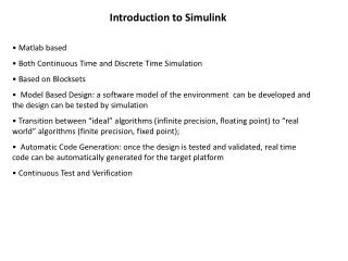
Configuration Parameters Notice the “Fixed-step size” of 0.1.
After Running the Simulation After clicking on “Autoscale”, it all appears to be working.
Aliasing Due to Insufficient Sampling After changing the “Fixed-step size” to 1 ... TOO LARGE!