Download

1 / 14
150 likes | 584 Views
Introduction to Matlab and Simulink. Dr Martin Brown E1k, Control Systems Centre School of Electrical and Electronic Engineering University of Manchester Tel: 0161 306 4672 martin.brown@manchester.ac.uk EEE Intranet. Background and Aims.

E N D
Introduction to Matlab and Simulink Dr Martin Brown E1k, Control Systems Centre School of Electrical and Electronic Engineering University of Manchester Tel: 0161 306 4672 martin.brown@manchester.ac.uk EEE Intranet
Background and Aims • Matlab and Simulink have become a defacto standard for system modelling, simulation and control • It is assumed that you know how to use these tools and develop Matlab and Simulink programs on this MSc. • Over the next two weeks, we’re going to have a rapid introduction to Matlab and Simulink covering: • Introduction to Matlab and help! • Matrix programming using Matlab • Structured programming using Matlab • System (and signal) simulation using Simulink • Modelling and control toolboxes in Matlab • Note that we’re not covering everything to do with Matlab and Simulink in these 4*2 hour lectures • Also, after every lecture block in this module, there is a 1 hour lab scheduled – programming is a practical activity
Resources • Mathworks Information • Mathworks: http://www.mathworks.com • Mathworks Central: http://www.mathworks.com/matlabcentral • http://www.mathworks.com/applications/controldesign/ • http://www.mathworks.com/academia/student_center/tutorials/launchpad.html • Matlab Demonstrations • Matlab Overview: A demonstration of the Capabilities of Matlab http://www.mathworks.com/cmspro/online/4843/req.html?13616 • Numerical Computing with Matlab http://www.mathworks.com/cmspro/online/7589/req.html?16880 • Select Help-Demos in Matlab • Matlab Help • Select “Help” in Matlab. Extensive help about Matlab, Simulink and toolboxes • Matlab Homework Helper http://www.mathworks.com/academia/student_center/homework/ • Newsgroup: comp.soft-sys.matlab • Matlab/Simulink student version (program and book ~£50) http://www.mathworks.com/academia/student_center • Other Matlab and Simulink Books • Mastering Matlab 6, Hanselman & Littlefield, Prentice Hall • Mastering Simulink 4, Dabney & Harman, Prentice Hall • Matlab and Simulink Student Version Release 14 • lots more on mathworks, amazon, …. It is important to have one reference book.
Introduction to Matlab • Click on the Matlab icon/start menu initialises the Matlab environment: • The main window is the dynamic command interpreter which allows the user to issue Matlab commands • The variable browser shows which variables currently exist in the workspace Command window Variable browser Command history
Matlab Programming Environment • Matlab (Matrix Laboratory) is a dynamic, interpreted, environment for matrix/vector analysis • Variables are created at run-time, matrices are dynamically re-sized, … • User can build programs (in .m files or at command line) using a C/Java-like syntax • Ideal environment for model building, system identification and control (both discrete and continuous time • Wide variety of libraries (toolboxes) available
Basic Matlab Operations • >> % This is a comment, it starts with a “%” • >> y = 5*3 + 2^2; % simple arithmetic • >> x = [1 2 4 5 6]; % create the vector “x” • >> x1 = x.^2; % square each element in x • >> E = sum(abs(x).^2); % Calculate signal energy • >> P = E/length(x); % Calculate av signal power • >> x2 = x(1:3); % Select first 3 elements in x • >> z = 1+i; % Create a complex number • >> a = real(z); % Pick off real part • >> b = imag(z); % Pick off imaginary part • >> plot(x); % Plot the vector as a signal • >> t = 0:0.1:100; % Generate sampled time • >> x3=exp(-t).*cos(t); % Generate a discrete signal • >> plot(t, x3, ‘x’); % Plot points
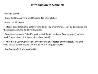
vs, vc t Introduction to Simulink • Simulink is a graphical, “drag and drop” environment for building simple and complex signal and system dynamic simulations. • It allows users to concentrate on the structure of the problem, rather than having to worry (too much) about a programming language. • The parameters of each signal and system block is configured by the user (right click on block) • Signals and systems are simulated over a particular time.
Starting and Running Simulink • Type the following at the Matlab command prompt • >> simulink • The Simulink library should appear • Click File-New to create a new workspace, and drag and drop objects from the library onto the workspace. • Selecting Simulation-Start from the pull down menu will run the dynamic simulation. Click on the blocks to view the data or alter the run-time parameters
Signals and Systems in Simulink • Two main sets of libraries for building simple simulations in Simulink: • Signals: Sources and Sinks • Systems: Continuous and Discrete
Basic Simulink Example • Copy “sine wave” source and “scope” sink onto a new Simulink work space and connect. • Set sine wave parameters modify to 2 rad/sec • Run the simulation: • Simulation - Start • Open the scope and leave open while you change parameters (sin or simulation parameters) and re-run • Many other Simulink demos …
Day 1: Matrix Programming in Matlab • Full notes/syntax will be recorded in the diary • Setting directory and diary • Simple maths • Matlab workspace, and help • Variables, comments, complex numbers and functions • Matlab desktop and management • Script m-files • Arrays • Creating and assigning arrays, standard arrays • Array indexing and orientation • Array operators • Array manipulation • Array sorting, sub-array searching and manipulation functions • Array size and memory utilization • Control structures • for and while loops • if else and switch decisions
Day 2: Structured Matlab Programming • Full notes/syntax will be recorded in the diary • Functions • Input and output arguments • File structure, search path • Exception handling • Debugging and profiling • Strings • Dynamic function and expression evaluation • Cell arrays • Data structures • Data plotting (2D/3D), figures • GUIDE • Simulink
Day 1: Laboratory • Remember • Change directory to your local filespace so that your work is saved • Turn on the diary on to save the commands and results from the lab session to a file for future reference • Questions • Use the help and lookfor commands and look at the normal Matlab help section in the pull down menu (F1). How does the sin() function work? • Evaluate expressions such as 7*8/9, 8^2, 6+5-3 • Using the in-built Matlab functions, evaluate sin(0), sin(pi/2), abs(-3) • Using the editor, write a Matlab script to solve the quadratic equation • 2x2 -10x + 12 = 0 • Evaluate, using a for loop, the first twenty numbers of the Fibonacci series • xn = xn-1 + xn-2, x0 = 1, x1 = 1 • Create the two vectors [1 2 3], [4 5 6] and calculate their inner product • Create the 3*3 matrix A = [1 2 3; 4 5 6; 7 8 9] and the column vector b = [1 2 3], and multiply the two together A*b. • Solve the equation A*x = b, where A and b are given in (6) • Modify (8), so that you neglect the 3rd row & column of information. • … http://www.facstaff.bucknell.edu/maneval/help211/exercises.html
Day 2: Laboratory • Write a function that returns the two roots of a quadratic equation, given the three arguments a, b and c. Test the function from the command line • Write a function that returns the mean and standard deviation of a vector of numbers (input vector). While Matlab supplies the mean() and std() functions, try just using the sum() and length() functions. • Write a function that reverses the order of letters in a string, and returns the new string. • Use the eval() Matlab function to evaluate strings such as: • exp1 = ‘5*6 + 7’; • Note this, and feval(), is very useful for dynamic programming • Use a cell array to store a list of expressions, stored as strings. Then use eval() and a for loop to iterate over the expressions and evaluate them. • Create two simple data structures to modify your solution to (1). Use one data structure to pack the parameters of the quadratic equation into a single variable, and use another to return the roots inside a single data structure • Create the vector 0:pi/20:2*pi and use it to sample the sin() function. Plot the results and edit the figure window to put labels on the figure. Save the figure (.fig) and export a .jpg file. • Use the meshgrid() function to sample a 2 dimensional input space between 0 and 2p, then use the data to sample the function sin(x1)*cos(x2). Plot the results using the mesh() function. • Create a GUI that prompts the user for a number and then displays double that number next to the entered value. • Start Simulink and using a sin()source and a scope sink, view the signal over 10 seconds. • Change the frequency of the sin() source and again compare the results. Next change the simulation length. • Build the first order system H(s) = 1/(1+3s) in the model and pass a sin() signal through the system. Make sure you run the simulation for a long enough time for the transients to die down and the system to settle. • Replace the first order system in (6) with the second order system, what is the difference when the system settles down H(s) = 1/(1+2s+s^2).