Download
1 / 26
260 likes | 425 Views
Lossy Compression of Images Corrupted by Mixed Poisson and Additive Gaussian Noise Vladimir V. Lukin a , Sergey S. Krivenko a , Mikhail S. Zriakhov a , Nikolay N. Ponomarenko a , Sergey K. Abramov a , Arto Kaarna b , Karen Egiazarian c

E N D
Lossy Compression of Images Corrupted by Mixed Poisson and Additive Gaussian Noise Vladimir V. Lukina, Sergey S. Krivenkoa, Mikhail S. Zriakhova, Nikolay N. Ponomarenkoa, Sergey K. Abramova, Arto Kaarnab, Karen Egiazarianc a National Aerospace University, 61070, Kharkov, Ukraine; b Lappeenranta University of Technology, Institute of Signal Processing, P.O. Box-20, FIN-53851, Lappeenranta , Finland; c Tampere University of Technology, Institute of Signal Processing, P.O. Box-553, FIN-33101, Tampere, Finland Lossy Compression of Images Corrupted by Mixed Poisson and Additive Gaussian Noise Vladimir Lukin
Contents • Contents • Introduction • Signal and Noise Models • Peculiarities of Lossy Compression of Noisy Images • Similarities and Differences Between Transform Based Filtering and Compression • Quantitative Criteria • Optimal Operation Point • Problems and Ways of Reaching OOP in Practice • Noise Removal Properties of Lossy Compression for Artificial Test Image • Noise Removal Properties of Lossy Compression for Real-life Test Images • Proposed Modified Procedure for Compressing Images Corrupted by Signal-dependent Noise • Conclusions Vladimir Lukin
Introduction • Applications: CCD color imaging systems, CCD multi- and hyper-spectral imaging systems • Goal: Analyzing main approaches to lossy compression with filtering effect of raw image data corrupted by mixed Poisson and additive Gaussian noise Reason: photon-counting image registration principle • Requirements (alternative): • essential compression ratios; • sufficient noise removal; • useful information preservation Color (multichannel) image Poisson noise CCD matrix Lossy compression techniques Additive noise Reason: instrumentation and ambient influences Achievement of the Optimal Operation Point (OOP) Vladimir Lukin
Signal and Noise Models defines an ij-th image pixel corrupted by Poisson noise with the true value equal to; defines zero-mean additive Gaussian noise with variance; I and J denote an image size. This model simulates real life situation of noise in R, G, and B components of color images under assumption that variance of fluctuations induced by Poisson noise for majority of image pixels is larger than variance of additive noise considered constant. The model also relates to other optical and infrared sensors like those ones applied in multi- and hyperspectral remote sensing imaging. Vladimir Lukin
Peculiarities of Lossy Compressionof Noisy Images Why lossy (not lossless) compression? • Lossy compression is able to provide considerably larger CRs (compared to lossless coding) without degrading image resolution and introducing disturbing artefacts; • A positive effect of image filtering can be observed due to lossy compression if introduced losses mainly relate to noise removal and useful image content is preserved. The RS (Helsinki region) image corrupted by additive Gaussian noise with σ2= 100 The decoded lossy compressed image (bpp = 0.75) Vladimir Lukin
Similarities and Differences Between Transform Based Filtering and Compression Similarity: In both orthogonal based filtering and compression, an image is subject to orthogonal transform applied either to entire image or locally, in blocks. Then, orthogonal transform coefficients are quantized in the case of image compression or thresholded if an image is denoised. Difference I: If hard thresholding is used, then for small amplitude coefficients that are assigned zero values there is no difference between quantization and denoising. But for large amplitude coefficients quantization used in lossy compression introduces losses in information content. Due to this, filtering observed in lossy compression of noisy images is always less efficient than denoising. Difference II: For improving performance of transform based denoising, a spatially invariant approach is used. Such approach is not and cannot be employed in compression. This is the second reason why filtering observed in lossy compression is less efficient than denoising. Vladimir Lukin
Quantitative Criteria The standard measures to characterize a compressed image quality - , where is the decompressed image; - - for 8 bits image representation. Alternative measures to characterize a compressed image quality - , where is the noise free image; - . It is more reasonable to characterize a compressed image quality by quantitative measures calculated with respect to the corresponding noise-free image (MSEnf, PSNRnf) rather than to the original noisy one (MSEor, PSNRor). Vladimir Lukin
Optimal Operation Point Optimal operation point (OOP): The argument of the curves MSEnf(CR), MSEnf(bpp) or MSEnf(QS) for which these curves reach theirs minima have been called optimal operation point (OOP): CROOP , bppOOP or QSOOP.. σ2 = 400 σ2 = 100 σ2 = 50 OOP is observed and commonly occurs to be more “obvious” for less complex content images and/or for rather intensive noise. Main idea: It is worth compressing a noisy image in the neighborhood of OOP. Main problem: In practice, noise-free image is not at disposal. Dependences MSEnf (QSn) for the noisy test gray-scale image Lena for different additive noise levels Vladimir Lukin
Problems and Ways of Reaching OOPin Practice Case I: pure additive noise Proposed procedure I:iteratively compressing/decompressing an image several times with calculating of standard MSE between original (noisy) and decompressed images.Using the interpolation of the obtained curve MSE(CR) (or MSE(bpp)) to determine an estimate of CROOP or bppOOP as such CR or bpp for which MSE was equal to variance of noise in original (noisy) image (a priori known or pre-estimated).* * N.N. Ponomarenko, V.V. Lukin, M.S. Zriakhov, and K. Egiazarian, “Lossy compression of images with additive noise”, in Proc. Intern. Conf. on Advanced Concepts for Intelligent Vision Systems, Belgium, 2005, pp. 381-386. Dependences of PSNRnf and PSNRor on bpp for the test gray-scale image Lena in conventional 8-bit representation for σ2=200 (PSNRor=25) Vladimir Lukin
Problems and Ways of Reaching OOPin Practice Case I: pure additive noise Proposed procedure II:for coders with CR controlled by quantization step QS (standard JPEG, AGU and ADCTC*, etc.). For such coders non-iterative procedure can be used. One has to set QSOOP approximately equal to 4.5σ where σ is a standard deviation of additive noise**. σ2 = 400 σ2 = 100 σ2 = 50 *http://www.ponomarenko.info/agu.htm and http://www.ponomarenko.info/adct.htm **N. Ponomarenko, V. Lukin, M. Zriakhov, K. Egiazarian, and J. Astola, “Estimation of accesible quality in noisy image compression”, in CD-ROM Proc. EUSIPCO, Italy, 2006, 4 p. Dependences MSEnf (QSn) for the noisy test gray-scale image Barbara for different additive noise levels Vladimir Lukin
Problems and Ways of Reaching OOPin Practice Case II: mixed additive and signal-dependent (multiplicative or Poisson) noise Possible strategies: • To apply lossy compression directly to an original image. • Problem I: it is difficult to recommend a way of setting parameters of a coder to provide compression in OOP neighbourhood. • Problem II: for multiplicative noise case more essential filtering effect of lossy compression was mainly observed for image regions with relatively small local means whilst for image regions with rather large local means noise was mainly not suppressed. • To apply a three-state compression. • At the first stage, the corresponding homomorphic transform is used, namely, of logarithmic type for pure multiplicative noise or Anscombe transform for compressing images corrupted by Poisson noise. • At the second stage, it becomes possible to apply known methods of compression. • At the third stage, decompressed images are subject to the corresponding inverse homomorphic transform. The question is what strategy is better? Vladimir Lukin
Noise Removal Properties of Lossy Compression for Artificial Test Image Test image: Artificial image of size 512x512 pixels has 16 vertical strips of width 32 pixels. For each strip, the values are the same, i.e. constant and equal to 20 (for the leftmost strip), 30, 40,…, 170. Peculiarities: After simulating noise ( ) the following conditions have been satisfied: and for any . The strip width suits well to operation principle of AGU coder that exploits just 32x32 pixel size of blocks. This allows minimizing blocking artifacts. For all strips (prevailing influence of signal-dependent noise for all strips and entire image). Artificial noisy test image Vladimir Lukin
Noise Removal Properties of Lossy Compression for Artificial Test Image(Strategy I: direct approach) To analyze noise suppression, we have determined residual variance for each l-th strip where is the is the true value for the l-th strip (equal to 10+10 l); It is also possible to analyze ratios to study noise suppression due to lossy compression quantitatively ( shows how many times noise variance has been reduced). For the coders AGU and SPIHT, we have obtained dependences of on l for several QS. The minimal QS was equal to whilst the maximal QS was about . Vladimir Lukin
Noise Removal Properties of Lossy Compression for Artificial Test Image(Strategy I: direct approach) Dependences of on l for different QSfor the coder AGU Dependences of on l for different bpp for the coder SPIHT Preliminary conclusion:For rather large bpp (quite small CR), small variance of residual noise is observed only for the leftmost strips (small l). If bpp becomes smaller, noise suppression increases ( reduces for all strips). Vladimir Lukin
Noise Removal Properties of Lossy Compression for Artificial Test Image(Strategy II: three-stage approach) Direct Anscombe-like Transform Inverse Anscombe-like Transform where DBI is the maximal value for a given image representation (e.g., 255 for 8 bits); denotes the decompressed image; defines rounding to the nearest integer. Note that compression is applied to the image . Inverse transform is carried out for an image after decompression. Small bias introduced by the pair of Anscombe-like transforms is neglected. For Poisson noise case, after applying the direct transform one gets an image corrupted by pure additive noise with practically constant variance . The presence of additive noise component in the considered model, although it is not predominant, changes the situation. Vladimir Lukin
Noise Removal Properties of Lossy Compression for Artificial Test Image(Strategy II: three-stage approach) For an l-th strip , where. Then if one has Variance is defined as ;since , one obtains This means that the image is corrupted by Gaussian noise with zero mean and variance which is equal for all pixels of the same strip but with variance slightly larger for strips with smaller l. Vladimir Lukin
Noise Removal Properties of Lossy Compression for Artificial Test Image(Strategy II: three-stage approach) Dependences of on l for different QSAfor the coder AGU Dependences of on l for different bpp for the coder SPIHT We can recommend to use QSA about 32…40 that produces almost constant of about 1…3 which is practically not seen in decompressed image (for the coder AGU). It is possible to provide very efficient noise suppression in image homogeneous regions if quantization step is set large enough or bpp is set small enough. If QS increases, residual noise from signal-dependent transforms to almost additive. Vladimir Lukin
Noise Removal Properties of Lossy Compression for Real-life Test Images Let us denote direct application of lossy compression, i.e., without the pair of Anscombe-like transforms as DC (direct compression). On the contrary, the compression procedure that exploits the Anscombe-like transforms will be denoted as HBC (homomorphic based compression). Real-life test image Airfield Real-life test image Frisco Vladimir Lukin
Noise Removal Properties of Lossy Compression for Real-life Test Images for both strategies, the coders AGU and SPIHT for the image Airfield for both strategies, the coders AGU and SPIHT for the image Frisco All obtained curves have maxima. For the image Airfield these maxima appear themselves less clearly than for the image Frisco. Maximal values for the image Frisco are larger than for the image Airfield. This is explained by less complex structure of information content for the image Frisco and the presence of rather large quasi-homogeneous regions in it. For more complex images curves maxima take place for larger bppOOP. Vladimir Lukin
Noise Removal Properties of Lossy Compression for Real-life Test Images It is possible to recommend using the HBC procedure for both coders. For the HBC procedure it is recommended to set fixed QSA about 35. The noisy real-life test image Frisco The compressed image (HBC strategy, AGU coder with QSA=35) Vladimir Lukin
Proposed Modified Procedure for Compressing Images Corrupted by Signal-dependent Noise Conclusion resulting from previous analysis: for efficient suppression of noise it is enough to have a lossy coder quantization step approximately equal to 4.5 standard deviations of noise in a given region. Main idea: instead of performing homomorphic transformations, it seems possible to set an appropriate individual QS for each particular image block if noise standard deviation for this block is a priori known or can be pre-estimated. Difficulties: It might seem that the use of specific (not equal) quantization steps for each block leads to necessity to save their values as side information at image coding stage. But this problem can be avoided. One thing we need before compressing an image is a priori known or pre-estimated dependence of local varianceon local mean . Vladimir Lukin
Proposed Modified Procedure for Compressing Images Corrupted by Signal-dependent Noise: Coding Stage The sequence of operations (for the AGU coder) performed for a given block: Calculate DCT in a block and obtain DCT coefficients ; Determine the block mean using ; for example, for DCT of size 32x32 pixels Quantize using quantization step QSD0 =10: (the value 10 is de- fined empirically in experiments); Reconstruct the block mean by multiplying by 10; Calculate quantization step QSDCT for other DCT coefficients (other than ) using known dependence as where k is a parameter to be ana-lyzed later (e.g., for the model of noise considered in this study ); Quantize all DCT coefficients of the given block and pass them to further coding. Vladimir Lukin
Proposed Modified Procedure for Compressing Images Corrupted by Signal-dependent Noise: Decoding Stage The sequence of operations (for the AGU coder) performed for a given block: Reconstruct a given block mean by multiplying by 10: ; Reconstruct ; for example, for 32x32 blocks ; Calculate quantization step QSDCT for other DCT coefficients taking into account that Reconstruct other than DCT coefficients of the given block using the decoded values and QSDCT for this block; Carry out inverse DCT in the block. Note: at the coding stage there is no need to code the values QSD0 and QSDCT for image blocks. At decoding stage, they are calculated using decoded values and known dependence of local variance on local mean. Vladimir Lukin
Proposed Modified Procedure for Compressing Images Corrupted by Signal-dependent Noise: Post-filtering Background: The coder AGU can use post-processing of decompressed images. Similar post-processing can be carried out for the proposed modification of the AGU coder (further denoted as AGU-M). Obtained results: Preliminary conclusion: The values of PSNRnf with post-filtering are better (larger) than the corresponding maximal values for the coding procedures considered earlier. Vladimir Lukin
Proposed Modified Procedure for Compressing Images Corrupted by Signal-dependent Noise: Pre-filtering Background: The quality of compressed images can be additionally improved if one uses image lossy compression with k considerably smaller than 4.5 with further post-filtering (for this strategy it was reasonable to set the parameter k ≈1.3). Obtained results: Preliminary conclusions: As it is seen, PSNRnf for the case of post-filtering has been improved. But this is reached by the expense of larger bpp, i.e., smaller CR provided. There is almost no difference in PSNRnf for k=1.0 and k=1.3. Then, it is reasonable to use k=1.3 since in this case larger CR values are provided. In practice, one has to decide what is of prime importance, larger PSNRnf or larger CR. Vladimir Lukin
Conclusions The task of compressing images corrupted by mixed Poisson and additive Gaussian noise is considered. It is shown that different approaches to compression are possible. All approaches result in some noise suppression due to lossy compression, i.e., to noise filtering. However, statistics of residual noise considerably depends upon a compression procedure used. It is demonstrated that more efficient ways are either to exploit root-square transforms (the use of Anscombe transform and its modifications will be considered in future) or to adjust coder parameters to statistical characteristics of mixed noise. It is possible to perform “careful” compression with small CR and then to carry out post-filtering. Image pre-filtering and lossy compression are possible as well. Recommendations concerning parameter selection for the considered approaches are presented. Vladimir Lukin