Image Denoising by OWT for Gaussian Noise Corrupted Images

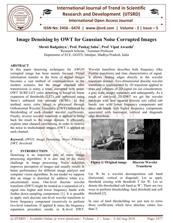
1. International Research Research and Development (IJTSRD) International Open Access Journal y OWT for Gaussian Noise Corrupted Images Shruti Badgainya1, Prof. Pankaj Sahu2, Prof. Vipul Awasthi Research Scholar, 2Assistant Professor f ECE, GGITS, Jabalpur, Madhya Pradesh, India International Journal of Trend in Scientific Scientific (IJTSRD) International Open Access Journal ISSN No: 2456 ISSN No: 2456 - 6470 | www.ijtsrd.com | Volume 6470 | www.ijtsrd.com | Volume - 2 | Issue – 5 Image Denoising by OWT or Gaussian Noise Corrupted Images Vipul Awasthi2 Shruti Badgainya 1Research Scholar, Department of ECE ABSTRACT In this paper denoising techniques for AWGN corrupted image has been mainly focused. Visual information transfer in the form of digital images becomes a vast method of communication in the modern scenario, but the image obtained after transmission is many a times corrupted with noise. OWT SURE-LET color denoising is based on linear expansion of thresholds (LET) and opti Stein’s unbiased risk estimate (SURE). In this method, noisy color image is processed through Orthonormal Wavelet Transform (OWT) followed by thresholding of each channel wavelet coefficients. Finally, inverse wavelet transform is applied to br back the result to the image domain. It efficiently exploits inter channel correlations. In order to remove the noise in multichannel images, OWT is applied on each channel. Keyword:AWGN, Image Denoising, Noise, Filtering, DWT, threshold. I INTRODUCTION Denoising is an important part of many image processing algorithms. It is also one of the main challenge in image processing. Noise reduction improves perception of images and usually results in better performance for different image analysis computer vision algorithms. In our model we suppose that an image is distorted by additive white (i.e. uncorrelated) noise. One-level discrete wavelet transform (DWT) might be treated as a separation of a signal into higher and lower frequency bands wi further down-sampling components [1]. It is possible to apply such discrete one-level wavelet transform to lower frequency component recursively to perform two-level transform. If applied K times the frequency separation procedure results in K separation procedure results in K-level DWT. Wavelet transform describes both frequency (like Fourier transform) and time characteristics of signal. It allows finding edges directly in the wavelet transform domain. Two-dimensional discrete wavelet transform is implemented by 1D transform applied rows and columns of 2D-signal (in our consideration, a gray scale image) separately and subsequently. As a result of one-level 2D-DWT we get the wavelet spectrum with four squared discrete sets called sub bands: one with lower frequency components and three sub bands with higher frequency components associated with horizontal, vertical and diagonals edge directions. In this paper denoising techniques for AWGN corrupted image has been mainly focused. Visual the form of digital images becomes a vast method of communication in the modern scenario, but the image obtained after transmission is many a times corrupted with noise. LET color denoising is based on linear expansion of thresholds (LET) and optimized using Stein’s unbiased risk estimate (SURE). In this method, noisy color image is processed through Orthonormal Wavelet Transform (OWT) followed by thresholding of each channel wavelet coefficients. Finally, inverse wavelet transform is applied to bring back the result to the image domain. It efficiently exploits inter channel correlations. In order to remove the noise in multichannel images, OWT is applied on Wavelet transform describes both frequency (like Fourier transform) and time characteristics of signal. It allows finding edges directly in the wavelet dimensional discrete wavelet transform is implemented by 1D transform applied to signal (in our consideration, scale image) separately and subsequently. As a DWT we get the wavelet spectrum with four squared discrete sets called sub bands: one with lower frequency components and bands with higher frequency components associated with horizontal, vertical and diagonals AWGN, Image Denoising, Noise, Filtering, Denoising is an important part of many image processing algorithms. It is also one of the main challenge in image processing. Noise reduction improves perception of images and usually results in better performance for different image analysis and computer vision algorithms. In our model we suppose that an image is distorted by additive white (i.e. Figure 1: Original image Discrete Wavelet Figure 1: Original image Discrete Wavelet Transform Let W be a wavelet decomposition sub (horizontal, vertical or diagonal). Let us apply threshold zeroing with threshold T for W. Let us denote the thresholded sub band as ways to perform thresholding: hard threshold and soft threshold [2]. In case of hard thresholding we just turn to zeros those coefficients which have absolute values less than T: a wavelet decomposition sub band (horizontal, vertical or diagonal). Let us apply threshold zeroing with threshold T for W. Let us level discrete wavelet band as W’. There are two transform (DWT) might be treated as a separation of a signal into higher and lower frequency bands with sampling components [1]. It is possible ways to perform thresholding: hard threshold and soft level wavelet transform to n case of hard thresholding we just turn to zeros those coefficients which have absolute values less lower frequency component recursively to perform level transform. If applied K times the frequency @ IJTSRD | Available Online @ www.ijtsrd.com @ IJTSRD | Available Online @ www.ijtsrd.com | Volume – 2 | Issue – 5| Jul-Aug 2018 Aug 2018 Page: 2477

2. International Journal of Trend in Scientific Research and Development (IJTSRD) ISSN: 2456 International Journal of Trend in Scientific Research and Development (IJTSRD) ISSN: 2456 International Journal of Trend in Scientific Research and Development (IJTSRD) ISSN: 2456-6470 Additive and Multiplicative Noises Additive and Multiplicative Noises Noise is present in an image either in an additive or multiplicative form. An additive noise follows the rule II.I Noise is present in an image either in an additive or multiplicative form. An additive noise follows the rule [9]: In case of soft thresholding we additionally pull down the absolute values of wavelet coefficients: In case of soft thresholding we additionally pull down absolute values of wavelet coefficients: While the multiplicative noise satisfies While the multiplicative noise satisfies Where s(x, y) is the original signal, n(x, noise introduced into the signal to produce the corrupted image w(x, y), and (x, pixel location. II.II Gaussian Noise Gaussian noise is evenly distributed over the signal this means that each pixel in the noisy image is the sum of the true pixel value and a random Gaussian distributed noise value. As the name indicates, this type of noise has a Gaussian distribution, whic bell shaped probability distribution function given by, bell shaped probability distribution function given by, y) is the original signal, n(x, y) denotes the noise introduced into the signal to produce the y), and (x, y) represents the Usually, soft thresholding shows better re sense, as opposed to hard thresholding. It is obvious that those wavelet coefficients that affect edges should be processed wiser and maybe even kept untouched during the thresholding. We propose an approach to retrieving that information by mask filters to wavelet decomposition coefficients using orthogonal wavelets. II. BASIC NOISE THEORY Noise is defined as an unwanted signal that interferes with the communication or measurement of another signal. A noise itself is an information- that conveys information regarding the sources of the noise and the environment in which it prop There are many types and sources of noise or distortions and they include [7][8]: Electronic noise such as thermal noise and shot noise. Acoustic noise emanating from moving, vibrating or colliding sources such as revolving machines, moving vehicles, keyboard clicks, wind and rain. Electromagnetic noise that can interfere with the transmission and reception of voice, image and data over the radio-frequency spectrum. Electrostatic noise generated by the presence of a voltage. Quantization noise and lost data packets due to network congestion. Signal distortion is the term often used to describe a systematic undesirable change in a signal and refers t changes in a signal from the non-ideal characteristics of the communication channel, signal fading reverberations, echo, and multipath reflections and missing samples. Depending on its frequency, spectrum or time characteristics, a noise process is further classified into several categories: er classified into several categories: Usually, soft thresholding shows better results in MSE It is obvious that those wavelet coefficients that affect edges should be processed wiser and maybe even kept untouched during the thresholding. We propose an approach to retrieving that information by applying mask filters to wavelet decomposition coefficients Gaussian noise is evenly distributed over the signal this means that each pixel in the noisy image is the sum of the true pixel value and a random Gaussian distributed noise value. As the name indicates, this type of noise has a Gaussian distribution, which has a Noise is defined as an unwanted signal that interferes with the communication or measurement of another Where g represents the gray level, m is the mean or average of the function and σ is the standard deviation of the noise. Graphically, it is represented as shown in Figure 1. When introduced into an image, Gaussian noise with zero mean and variance as 0.05 as in Figure 1 [3]. -bearing signal Where g represents the gray level, m is the mean or average of the function and σ is the standard deviation of the noise. Graphically, it is represented as shown in Figure 1. When introduced into an image, Gaussian noise with zero mean and variance as 0.05 would look that conveys information regarding the sources of the noise and the environment in which it propagates. There are many types and sources of noise or such as thermal noise and shot emanating from moving, vibrating or colliding sources such as revolving machines, moving vehicles, keyboard clicks, wind that can interfere with the transmission and reception of voice, image and ncy spectrum. by the presence of Figure 1: (a) Gaussian noise (mean=0, variance Figure 1: (a) Gaussian noise (mean=0, variance 0.05), (b) Gaussian distribution 0.05), (b) Gaussian distribution II.III Salt and Pepper Noise Salt and pepper noise is an impulse type of noise, which is also referred to as intensity spikes. This is caused generally due to errors in data transmission. It has only two possible values, of each is typically less than 0.1. The corrupted pixels are set alternatively to the minimum or to the maximum value, giving the image a “salt and pepper” like appearance. Unaffected pixels remain unchanged. For an 8-bit image, the typical bit image, the typical value for pepper noise and lost data packets due to Salt and Pepper Noise Salt and pepper noise is an impulse type of noise, which is also referred to as intensity spikes. This is aused generally due to errors in data transmission. It has only two possible values, a and b. The probability of each is typically less than 0.1. The corrupted pixels are set alternatively to the minimum or to the maximum value, giving the image a “salt and pepper” like appearance. Unaffected pixels remain unchanged. Signal distortion is the term often used to describe a systematic undesirable change in a signal and refers to ideal characteristics of the communication channel, signal fading reverberations, echo, and multipath reflections and missing samples. Depending on its frequency, spectrum or time characteristics, a noise process is @ IJTSRD | Available Online @ www.ijtsrd.com @ IJTSRD | Available Online @ www.ijtsrd.com | Volume – 2 | Issue – 5| Jul-Aug 2018 Aug 2018 Page: 2478

3. International Journal of Trend in Scientific Research and Development (IJTSRD) ISSN: 2456 International Journal of Trend in Scientific Research and Development (IJTSRD) ISSN: 2456 International Journal of Trend in Scientific Research and Development (IJTSRD) ISSN: 2456-6470 is 0 and for salt noise 255. The salt and pepper noise is generally caused by malfunctioning of pixel elements in the camera sensors, faulty memory locations, or timing errors in the digitization process. The probability density function for this type of noise is shown in Figure 2. is 0 and for salt noise 255. The salt and pepper noise is generally caused by malfunctioning of pixel elements in the camera sensors, faulty memory locations, or timing errors in the digitization process. II.V Brownian Noise Brownian noise comes under the category of fractal or 1/f noises. The mathematical model for 1/ fractional Brownian motion. Fractal Brownian motion is a non-stationary stochastic process that follows a normal distribution. Brownian noise is a special case of 1/f noise. It is obtained by integrating white noise. It can be graphically represented as shown in Figure 5. On an image, Brownian noise would look like Image 6. Brownian noise comes under the category of fractal or noises. The mathematical model for 1/f noise is fractional Brownian motion. Fractal Brownian motion stationary stochastic process that follows a normal distribution. Brownian noise is a special case noise. It is obtained by integrating white noise. It can be graphically represented as shown in Figure 5. On an image, Brownian noise would look like ction for this type of noise Figure 2: (a) Salt and pepper noise (b) PDF for salt and pepper noise Figure 2: (a) Salt and pepper noise (b) PDF for II.IV Speckle Noise Speckle noise is a multiplicative noise. This type of noise occurs in almost all coherent imaging systems such as laser, acoustics and SAR (Synthetic Aperture Radar) imagery. The source of this noise is attributed to random interference between the coherent returns. Fully developed speckle noise has the characteristic of multiplicative noise. Speckle noise foll distribution and is given as: Speckle noise is a multiplicative noise. This type of noise occurs in almost all coherent imaging systems uch as laser, acoustics and SAR (Synthetic Aperture Radar) imagery. The source of this noise is attributed to random interference between the coherent returns. Fully developed speckle noise has the characteristic of multiplicative noise. Speckle noise follows a gamma Fig. 5: Brownian noise distribu Fig. 5: Brownian noise distribution Where variance is a2α and g is the gray level. On an image, speckle noise (with variance 0.05) looks as shown in Figure 3 is the gray level. On an image, speckle noise (with variance 0.05) looks Fig. 6: Brownian noise Fig. 6: Brownian noise III. III.I Linear and Nonlinear Filtering Approach Filters play a major role in the image restoration process. The basic concept behind image restoration using linear filters is digital convolution and moving window principle. Let w(x) be the input signal subjected to filtering, and z(x) be the filtered output. If the filter satisfies certain conditions such as linearity and shift invariance, then the output filter can be expressed mathematically in simple form as expressed mathematically in simple form as DENOISING APPROACH DENOISING APPROACH Linear and Nonlinear Filtering Approach Filters play a major role in the image restoration process. The basic concept behind image restoration using linear filters is digital convolution and moving Fig. 3: Speckle noise ) be the input signal ) be the filtered output. If The gamma distribution is given below in Figure 4 The gamma distribution is given below in Figure 4 the filter satisfies certain conditions such as linearity and shift invariance, then the output filter can be Where h(t) is called the point spread function or impulse response and is a function that completely characterizes the filter. The integral represents a convolution integral and, in short, can be expressed as z = w* h ) is called the point spread function or nd is a function that completely characterizes the filter. The integral represents a convolution integral and, in short, can be expressed as Fig. 4: Gamma distribution 4: Gamma distribution h. @ IJTSRD | Available Online @ www.ijtsrd.com @ IJTSRD | Available Online @ www.ijtsrd.com | Volume – 2 | Issue – 5| Jul-Aug 2018 Aug 2018 Page: 2479

4. International Journal of Trend in Scientific Research and Development (IJTSRD) ISSN: 2456 International Journal of Trend in Scientific Research and Development (IJTSRD) ISSN: 2456 International Journal of Trend in Scientific Research and Development (IJTSRD) ISSN: 2456-6470 For a discrete case, the integral turns into a summation as For a discrete case, the integral turns into a stationary images, i.e., images that have abrupt changes in intensity. Such filters are known for their ability in automatically tracking an nce or when a signal is variable with little a priori knowledge about the signal to be processed. In general, an adaptive filter iteratively adjusts its parameters during scanning the image to match the image generating mechanism. This gnificant in practical images, stationary. denoising non-stationary images, i.e., images that have abrupt changes in intensity. Such filters are known for their ability in automatically tracking an unknown circumstance or when a signal is variable with little a priori knowledge about the signal to be processed. In general, an adaptive filter iteratively adjusts its parameters during scanning the image to match the image generating mechanism. This mechanism is more significant in practical images, which tend to be non-stationary. Compared to other adaptive filters, the Least Mean Square (LMS) adaptive filter is known for its simplicity in computation and implementation. The basic model is alinear combination of a low-pass image and a non component through a weighting function. Thus, the function provides compromise between resolution of genuine features and suppression of noise. The LMS adaptive filter incorporating a local mean estimator works on the following concept. A window, W, of size m×n is scanned over the image. The mean of this window, μ, is subtracted from the elements in the window to get the residual matrix W r=W – III.IV Median Filter A median filter belongs to the class of nonlinear filters unlike the mean filter. The median filter also follows the moving window principle similar to the mean filter. A 3× 3, 5× 5, or 7× 7 kernel of pixels is scanned over pixel matrix of the entire image. The median of the pixel values in the window is computed, and the center pixel of the window is replaced with the computed median. Median filtering is done by, first sorting all the pixel values from the surrounding neighborhood into numerical order and then replacing the pixel being considered with the middle pixel value. Note that the median value must be written to a separate array or buffer so that the results are not corrupted as the process is performed. results are not corrupted as the process is performed. III.II MEAN FILTER A mean filter acts on an image by smoothing it; that is, it reduces the intensity variation between adjacent pixels. The mean filter is nothing but a simple sliding window spatial filter that replaces the center value in the window with the average of all the neighboring pixel values including itself. By doing this, it replaces pixels that are unrepresentative of their surroundings. It is implemented with a convolution mask, which provides a result that is a weighted sum of the values of a pixel and its neighbors. It is also called a linear filter. The mask or kernel is a square. Often a 3× 3 square kernel is used. If the coefficients of the mask sum up to one, then the average brightness of the image is not changed. If the coefficients sum to zero, the average brightness is lost, and it returns a dark image. The mean or average filter works on the shift multiply-sum principle this principle in the two dimensional image can be represented as shown below: A mean filter acts on an image by smoothing it; that is, it reduces the intensity variation between adjacent pixels. The mean filter is nothing but a simple sliding window spatial filter that replaces the center value in the neighboring Compared to other adaptive filters, the Least Mean Square (LMS) adaptive filter is known for its simplicity in computation and implementation. The basic model is alinear combination of a stationary pass image and a non-stationary high-pass component through a weighting function. Thus, the function provides compromise between resolution of genuine features and suppression of noise. . By doing this, it replaces pixels that are unrepresentative of their surroundings. It is implemented with a convolution mask, which provides a result that is a weighted sum of the values ghbors. It is also called a linear filter. The mask or kernel is a square. Often a 3× 3 square kernel is used. If the coefficients of the mask sum up to one, then the average brightness of the image is not changed. If the coefficients sum to zero, age brightness is lost, and it returns a dark image. The mean or average filter works on the shift- sum principle this principle in the two- dimensional image can be represented as shown The LMS adaptive filter incorporating a local mean timator works on the following concept. A window, is scanned over the image. The mean of this window, μ, is subtracted from the elements in the window to get the residual matrix Wr. –μ to the class of nonlinear filters unlike the mean filter. The median filter also follows the moving window principle similar to the mean filter. A 3× 3, 5× 5, or 7× 7 kernel of pixels is scanned over pixel matrix of the entire image. The el values in the window is computed, and the center pixel of the window is replaced with the computed median. Median filtering is done by, first sorting all the pixel values from the surrounding neighborhood into numerical order and l being considered with the middle pixel value. Note that the median value must be written to a separate array or buffer so that the Fig. 7: Filter mask It should be observed that the coefficients of this mask sum to one, so the image brightness is retained, and the coefficients are all positive, so it will tend to blur the image. Mean filters are popular for their simplicity and ease of implementation. Th filter is used in applications where the noise in certain regions of the image needs to be removed. In other words, the mean filter is useful when only a part of the image needs to be processed. III.III LMS Adaptive Filter An adaptive filter does a better job of denoising images compared to the averaging filter. The fundamental difference between the mean filter and the adaptive filter lies in the fact that the weight matrix varies after each iteration in the adaptive filter while it remains constant throughout the iterations in the mean filter. Adaptive filters are capable of the mean filter. Adaptive filters are capable of It should be observed that the coefficients of this mask sum to one, so the image brightness is retained, and the coefficients are all positive, so it will tend to blur the image. Mean filters are popular for their simplicity and ease of implementation. The mean filter is used in applications where the noise in certain regions of the image needs to be removed. In other words, the mean filter is useful when only a part of es a better job of denoising images compared to the averaging filter. The fundamental difference between the mean filter and the adaptive filter lies in the fact that the weight matrix varies after each iteration in the adaptive filter stant throughout the iterations in Fig 8: Concept of median filtering Fig 8: Concept of median filtering @ IJTSRD | Available Online @ www.ijtsrd.com @ IJTSRD | Available Online @ www.ijtsrd.com | Volume – 2 | Issue – 5| Jul-Aug 2018 Aug 2018 Page: 2480

5. International Journal of Trend in Scientific Research and Development (IJTSRD) ISSN: 2456 International Journal of Trend in Scientific Research and Development (IJTSRD) ISSN: 2456 International Journal of Trend in Scientific Research and Development (IJTSRD) ISSN: 2456-6470 Neighborhood values: 115, 119, 120, 123, 126, 127, 150 Median value: 124 The central pixel value of 150 in the 3×3 window shown in Figure 8 is rather unrepresentative of the surrounding pixels and is replaced with the median value of 124. The median is more robust compar the mean. Thus, a single very unrepresentative pixel in a neighborhood will not affect the median value significantly. Since the median value must actually be the value of one of the pixels in the neighborhood, the median filter does not create new unrealistic pixel values when the filter straddles an edge. For this reason the median filter is much better at preserving sharp edges than the mean filter. These advantages aid median filters in denoising uniform noise as well from an image. III.V Discrete Wavelet Transform (DWT) Wavelets are mathematical functions that analyze data according to scale or Resolution. They aid in studying a signal in different windows or at different resolutions. For instance, if the signal is viewed in a large window, gross features can be noticed, but if viewed in a small window, only small features can be noticed. Wavelets provide some advantages over Fourier transforms. For example, they do a good job in approximating signals with sharp spikes or signals having discontinuities. Wavelets can also model speech, music, video and non-stationary stochastic signals. Wavelets can be used in applications such as image compression, turbulence, human vision, radar, earthquake prediction, etc. The term “wavelets” is used to refer to a set of Ortho-normal basis functions generated by dilation and translation of scaling function φ and a mother wavelet ψ. The finite scale multi resolution representation of a discrete function can be called as a discrete wavelet transform. DWT is a fast linear operation on a data vector, whose length is an integer power of 2. This transform is invertible and orthogonal, where the inverse transform expressed as a matrix is the transpose of the transform matrix. The wavelet basis or function, unlike sine cosines as in Fourier transform, is quite localized in space. But similar to sine and cosines, individual wavelet functions are localized in frequency. The Ortho-normal basis or wavelet basis is defined as: normal basis or wavelet basis is defined as: 123, 124, 125, e ψ is called the wavelet function and j and k are integers that scale and dilate the wavelet function. ‟ is known as the scale index, which ‟s width. The location index k provides the position. The wavelet function is dilated by powers of two and is translated by the integer k. In terms of the wavelet coefficients, the wavelet equation Where ψ is called the wavelet function and j and k are integers that scale and dilate the wavelet function. The factor „j‟ is known as the scale index, which indicates the wavelet‟s width. The location index k provides the position. The wavelet function is dil by powers of two and is translated by the integer k. In terms of the wavelet coefficients, the wavelet equation is The central pixel value of 150 in the 3×3 window shown in Figure 8 is rather unrepresentative of the surrounding pixels and is replaced with the median value of 124. The median is more robust compared to the mean. Thus, a single very unrepresentative pixel in a neighborhood will not affect the median value significantly. Since the median value must actually be the value of one of the pixels in the neighborhood, the Where g0, g1, g2,…. are high pass wavelet coefficients. Writing the scaling equation in terms of the scaling coefficients as given below, we get the scaling coefficients as given below, we get Where g0, g1, g2,…. are high pass wavelet coefficients. Writing the scaling equation in terms of nrealistic pixel values when the filter straddles an edge. For this reason the median filter is much better at preserving sharp edges than the mean filter. These advantages aid median filters in denoising uniform noise as well from ete Wavelet Transform (DWT) Wavelets are mathematical functions that analyze data according to scale or Resolution. They aid in studying a signal in different windows or at different resolutions. For instance, if the signal is viewed in a oss features can be noticed, but if viewed in a small window, only small features can be noticed. Wavelets provide some advantages over Fourier transforms. For example, they do a good job in approximating signals with sharp spikes or signals inuities. Wavelets can also model Fig.9: A 1-Dimensional DWT Dimensional DWT - Decomposition step DWT is the multi resolution description of an image. ecoding can be processed sequentially from a low resolution to the higher resolution. DWT splits the signal into high and low frequency parts. The high frequency part contains information about the edge components, while the low frequency part is split in into high and low frequency parts. The high frequency components watermarking since the human eye is less sensitive to changes in edges. In two dimensional applications, for each level of decomposition, we first perform the he vertical direction, followed by the DWT in the horizontal direction. After the first level of decomposition, there are 4 sub-bands: LL1, LH1, HL1, and HH1. For each successive level of DWT is the multi resolution description of an image. The decoding can be processed sequentially from a low resolution to the higher resolution. DWT splits the signal into high and low frequency parts. The high frequency part contains information about the edge components, while the low frequency part is split again into high and low frequency parts. The high frequency components watermarking since the human eye is less sensitive to changes in edges. In two dimensional applications, for each level of decomposition, we first perform the DWT in the vertical direction, followed by the DWT in the horizontal direction. After the first level of decomposition, there are 4 sub HL1, and HH1. For each successive level of decomposition, the LL Sub-band of the previous level is used as the input. To perform second level decomposition, the DWT is applied to LL1 band which decomposes the LL1 band into the four sub bands LL2, LH2, HL2, and HH2. To perform third level decomposition, the DWT is applied to LL2 band which decompose this band i the four sub-bands – LL3, LH3, HL3, HH3. This LL3, LH3, HL3, HH3. This stationary stochastic signals. Wavelets can be used in applications such as image compression, turbulence, human vision, radar, earthquake prediction, etc. The term “wavelets” is normal basis functions are are usually usually used used for for generated by dilation and translation of scaling function φ and a mother wavelet ψ. The finite scale multi resolution representation of a discrete function can be called as a discrete wavelet transform. DWT is t linear operation on a data vector, whose length is an integer power of 2. This transform is invertible and orthogonal, where the inverse transform expressed as a matrix is the transpose of the transform matrix. The wavelet basis or function, unlike sine and cosines as in Fourier transform, is quite localized in space. But similar to sine and cosines, individual wavelet functions are localized in frequency. The band of the previous level input. To perform second level decomposition, the DWT is applied to LL1 band which decomposes the LL1 band into the four sub- bands LL2, LH2, HL2, and HH2. To perform third level decomposition, the DWT is applied to LL2 band which decompose this band into The scaling function is given as: @ IJTSRD | Available Online @ www.ijtsrd.com @ IJTSRD | Available Online @ www.ijtsrd.com | Volume – 2 | Issue – 5| Jul-Aug 2018 Aug 2018 Page: 2481

6. International Journal of Trend in Scientific Research and Development (IJTSRD) ISSN: 2456-6470 results in 10 sub-bands per component. LH1, HL1, and HH1 contain the highest frequency bands present in the image tile, while LL3 contains the lowest frequency band. DWT is currently used in a wide variety of signal processing applications, such as in audio and video compression, removal of noise in audio, and the simulation of wireless antenna distribution. The choice of a threshold is an important point of interest. It plays a major role in the removal of noise in images because denoising most frequently produces smoothed images, reducing the sharpness of the image. Care should be taken so as to preserve the edges of the denoised image. There exist various methods for wavelet thresholding, which rely on the choice of a threshold value. Some typically used methods for image noise removal include VisuShrink, Sure Shrink and BayesShrink. Prior to the discussion of these methods, it is necessary to know about the two general categories of thresholding. They are hard- thresholding and soft-thresholding types. V. PROPOSED METHODOLOGY Fig. 10: 3 level discrete wavelet decomposition Wavelets have their energy concentrated in time and are well suited for the analysis of transient, time- varying signals. Since most of the real life signals encountered are time varying in nature, the Wavelet Transform suits many applications very well. As mentioned earlier, the wavelet equation produces different wavelet families like Daubechies, Haar, Coiflets, etc. The filter lengths and the number of vanishing moments for four different wavelet families are tabulated in Table 1. Table 1: Wavelet families and their properties IV. WAVELET THRESHOLDING The term wavelet thresholding is explained as decomposition of the data or the image into wavelet coefficients, comparing the detail coefficients with a given threshold value, and shrinking these coefficients close to zero to take away the effect of noise in the data. The image is reconstructed from the modified coefficients. This process is also known as the inverse discrete wavelet transform. During thresholding, a wavelet coefficient is compared with a given threshold and is set to zero if its magnitude is less than the threshold; otherwise, it is retained or modified depending on Thresholding distinguishes between the coefficients due to noise and the ones consisting of important signal information. Fig. 11: Proposed Algorithm VI. In this work we have taken ‘camerman’ standard test image for testing our proposed algorithm. Simulation results are: Symlet8 Wavelet is Selected Enter the value of Noise Varience (Sigma in dB): 10 AWGN Noise added with Varience (Sigma): 10.00 [dB] Input Noisy Image MSE: 100.01 Input Noisy Image PSNR: 28.13 [dB] Denoised by Proposed OWT-SURE MSE: 37.85 Denoised by Proposed OWT-SURE PSNR: 32.35 [dB] The SSIM value of Denoised Image: 0.8834 SIMULATION RESULTS the threshold rule. @ IJTSRD | Available Online @ www.ijtsrd.com | Volume – 2 | Issue – 5| Jul-Aug 2018 Page: 2482

7. International Journal of Trend in Scientific Research and Development (IJTSRD) ISSN: 2456 International Journal of Trend in Scientific Research and Development (IJTSRD) ISSN: 2456 International Journal of Trend in Scientific Research and Development (IJTSRD) ISSN: 2456-6470 5.Wangmeng Zuo et-al, “Gradient Histogram Estimation and Preservation for Texture Enhanced Image Denoising”, IEEE Transactions on Imag Processing, Volume 23, Number 6, June 2014. Processing, Volume 23, Number 6, June 2014. Elapsed time: 0.34 [sec] al, “Gradient Histogram Estimation and Preservation for Texture Enhanced Image Denoising”, IEEE Transactions on Image 6.Twinkle Shah et-al, “Epitome based Transform domain Image Denoising”, Published in IEEE, IET Image Processing Magazine, Pp. 71 2015. al, “Epitome based Transform domain Image Denoising”, Published in IEEE, IET Image Processing Magazine, Pp. 71 – 79, Fig. 12: Simulation Result for Cameraman image Fig. 12: Simulation Result for Cameraman image V. In this paper image denoising techniques for the AWGN corrupted has been given. This paper reviews the existing denoising algorithms, such as filtering approach; wavelet based approach. Different noise models including additive and multiplicative types ar used. The wavelet based approach finds applications in denoising images corrupted with Gaussian noise. Selection of the denoising algorithm is application dependent. OWT SURE-LET color denoising is based on linear expansion of thresholds (LET) and optimized using Stein’s unbiased risk estimate (SURE). In this method, noisy color image is processed through Orthonormal Wavelet Transform (OWT) followed by thresholding of each channel wavelet coefficients. Finally, transform is applied to bring back the result to the image domain. It efficiently exploits inter channel correlations. In order to remove the noise in multichannel images, OWT is applied on each channel. REFERENCES 1.Maxim Kimlyk et-al, “Image Denoising Using Discrete Wavelet Information”, IEEE Conference of Russian Young Researchers in Electrical Engineering (EIConRus), 2018. 7.De-An Huang et-al, “Self Decomposition with Applications to Single Image Denoising”, IEEE Transaction on Multimedia, Volume 16, Number 01, 2014. Volume 16, Number 01, 2014. al, “Self-Learning Based Image Applications to Single Image CONCLUSION In this paper image denoising techniques for the AWGN corrupted has been given. This paper reviews the existing denoising algorithms, such as filtering approach; wavelet based approach. Different noise models including additive and multiplicative types are used. The wavelet based approach finds applications in denoising images corrupted with Gaussian noise. Selection of the denoising algorithm is application LET color denoising is based on linear expansion of thresholds (LET) and zed using Stein’s unbiased risk estimate (SURE). In this method, noisy color image is processed through Orthonormal Wavelet Transform (OWT) followed by thresholding of each channel wavelet coefficients. Finally, Denoising”, IEEE Transaction on Multimedia, 8.Ajay Boyat et-al, “Image Denoising using Wavelet Transform and Median Filtering”, Nirma University IEEE International Conference on Engineering (NUiCONE), Engineering (NUiCONE), 2013. al, “Image Denoising using Wavelet Transform and Median Filtering”, Nirma University IEEE International Conference on 9.Paras Jain & Vipin Tyagi, “Spatial and frequency domain filters for restoration of noisy images”, IETE Journal of Education, 54(2), 108 IETE Journal of Education, 54(2), 108-116, 2013. Paras Jain & Vipin Tyagi, “Spatial and frequency domain filters for restoration of noisy images”, 10.Maggioni, M., Katkovnik, V., Egiazarian, K., Foi, “A.: Nonlocal transform volumetric data denoising and reconstruction”, IEEE Transaction on Image Processing, 22(1), 119–133, 2013. Maggioni, M., Katkovnik, V., Egiazarian, K., Foi, “A.: Nonlocal transform-domain data denoising and reconstruction”, IEEE Transaction on Image Processing, 22(1), filter for inverse inverse wavelet wavelet g back the result to the image domain. It efficiently exploits inter channel correlations. In order to remove the noise in multichannel images, OWT is applied on each 11.Silva, R.D., Minetto, R., Schwartz, W.R., Pedrini, H.: Adaptive edge-preserving image denoising using wavelet transforms. Pattern Analysis and Applications. Springer, 10.1007/s10044-012-0266 0266-x, 2012. Silva, R.D., Minetto, R., Schwartz, W.R., Pedrini, preserving image denoising using wavelet transforms. Pattern Analysis and inger, Berlin Berlin doi doi: 12.Zhang, Y., Li, C., Jia, J, “Image denoising using an improved bivariate threshold function in tetrolet domain”, 2013. Zhang, Y., Li, C., Jia, J, “Image denoising using an improved bivariate threshold function in al, “Image Denoising Using rm Transform and and Edge Edge Information”, IEEE Conference of Russian Young Researchers in Electrical and and Electronic Electronic 13.Dai, L., Zhang, Y., Li, Y.: Image denoising using BM3D combining tetrolet prefiltering Technol. J. 12(10), 1995–2001, 2013. Dai, L., Zhang, Y., Li, Y.: Image denoising using BM3D combining tetrolet prefiltering. Inf. 2001, 2013. 2.[2] S. Routray et-al, “A Novel Study on Color Image Denoising and Comparison of Various State-of-the-art Methods”, IEEE Intern Conference on Trends in Electronics and Informatics (ICEI) 2017. al, “A Novel Study on Color Image Denoising and Comparison of Various art Methods”, IEEE International Conference on Trends in Electronics and 14.He, K., Sun, J., Tang, X.: Guided image filtering. In: Proceedings European Computer Vision, pp. 1–14, 2010. He, K., Sun, J., Tang, X.: Guided image filtering. In: Proceedings European 14, 2010. Conference Conference on on 15.Porikli, F, “Constant time O(1) bilateral filtering”, In Proceeding IEEE Conference on Co Vision and Pattern Recognition, Anchorage, pp. 1–8, 2008. Porikli, F, “Constant time O(1) bilateral filtering”, In Proceeding IEEE Conference on Computer Vision and Pattern Recognition, Anchorage, pp. 3.S.H. Ismael et-al, “A New Approach of Image Denoising Based Transform”, IEEE World Computer Applications & Research, 2016. Computer Applications & Research, 2016. al, “A New Approach of Image Based Discrete IEEE Denoising Transform”, on on World Discrete Symposium Symposium Wavelet Wavelet on on 16.Yang, Q., Tan, K.H., Ahuja, N, “Real bilateral filtering”, Conference on Computer Vision and Pattern Recognition, Miami, pp. 557 Recognition, Miami, pp. 557–564, 2009. Yang, Q., Tan, K.H., Ahuja, N, “Real-time O(1) bilateral filtering”, Conference on Computer Vision and Pattern 4.Liqiang Shi, “An Improved Image Denoising Algorithm”, Seventh Conference on Measuring Technology and Mechatronics Automation, 2015. mage Denoising In In Proceedings Proceedings IEEE IEEE Algorithm”, Conference on Measuring Technology and Seventh IEEE IEEE International International @ IJTSRD | Available Online @ www.ijtsrd.com @ IJTSRD | Available Online @ www.ijtsrd.com | Volume – 2 | Issue – 5| Jul-Aug 2018 Aug 2018 Page: 2483

8. International Journal of Trend in Scientific Research and Development (IJTSRD) ISSN: 2456-6470 17.Farbman, Z., Fattal, R., Lischinski, D., Szeliski, “R.: Edge-preserving decompositions for multi- scale tone and detail manipulation”, ACM Transactions on Graphics 27(3), 1–10, 2008. filtering. In: SPIE electronic imaging: algorithms and systems, vol. 6064, pp. 606414-1–606414-12, 2006. 23.Yuan, X., Buckles, B.: Sub band noise estimation for adaptive wavelet shrinkage. In: Proceeding 17th International Conference Recognition, vol. 4, pp 885–888, 2004. 18.Paris, S., Durand, F, “A fast approximation of the bilateral filter using signal processing approach”, In the Proceeding of European Conference on Computer Vision, pp. 568–580, 2006. on Pattern 24.Elad, M.: On the origin of the bilateral filter and ways to improve it. IEEE Transaction Image Processing, 11(10), 1141–1151, 2002. 19.Gonzalez, R.C., Woods, R.E.: Digital image processing, 3rd edn. Prentice-Hall, Upper Saddle River, 2008. 25.Sendur, L., Selesnick, I. W.: Bivariate shrinkage functions for wavelet-based denoising exploiting inter scale dependency. IEEE Trans. Signal Process. 50(11), 2744–2756, 2002. 20.Blu, T., Luisier, F, “The SURE-LET approach to image denoising”, IEEE Transaction Image Processing, 16(11), 2778–2786, 2007. 21.Paris, S., Durand, F.: A fast approximation of the bilateral filter using signal processing approach. In: Proceeding European Conference on Computer Vision, pp. 568–580, 2006. 26.Chang, S., Yu, B., Vetterli, M.: Spatially adaptive wavelet thresholding based on context modeling for image denoising. IEEE Trans. Image Process. 9(9), 1522–1531, 2000. 22.Dabov, K., Foi, A., Katkovnik, V., Egiazarian, K.: Image denoising with block-matching and 3D @ IJTSRD | Available Online @ www.ijtsrd.com | Volume – 2 | Issue – 5| Jul-Aug 2018 Page: 2484