Lossy Compression
E[X(i,j)X(i-1,j)] E[X 2 (i,j)]. E[X(i,j)X(i,j-1)] E[X 2 (i,j)]. Lossy Compression. Based on spatial redundancy Measure of spatial redundancy: 2D covariance Cov X (i,j)= 2 e - a (i*i+j*j) Vertical correlation r 1 = Horizontal correlation r 2 = For images we assume equal correlations

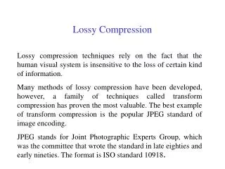
Lossy Compression
E N D
Presentation Transcript
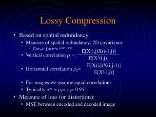
E[X(i,j)X(i-1,j)] E[X2(i,j)] E[X(i,j)X(i,j-1)] E[X2(i,j)] Lossy Compression • Based on spatial redundancy • Measure of spatial redundancy: 2D covariance • CovX(i,j)= 2e-a(i*i+j*j) • Vertical correlation r1= • Horizontal correlation r2= • For images we assume equal correlations • Typically e-a=r1= r2= 0.95 • Measure of loss (or distortion): • MSE between encoded and decoded image
Rate-Distortion Function • Tradeoff between bit rate (R) of compressed image and distortion (D) • R measured in its per encoder output symbol • Compression ratio = encoder input bits/R • D normalized by the variance of the encoder input • Possible SNR definition = 10 log10 D-1 • For images that can be modeled as uncorrelated Gaussian • R(D)=0.5log2 D-1 • More realistic images • See graph • How do you make these graphs?
Sample vs. Block-based Coding • Sample-based • In spatial or frequency domain • Like the JPEG-LS • Make a predictor function (often weighted sum) • Compute and quantize residual • Encode • Block-based • Spatial: group pixels into blocks, compress blocks • Transform: group into blocks, transform, encode
Which Transformation? • Considerations • Packing the most energy in the least number of elements • Minimizing the total entropy of the sequence • Decorrelating elements in the input blocks maximally • Coding complexity • DFT, KLT, DCT, DHT? See the effects • DCT-based coding • High compaction efficiency for correlated data • Orthogonal and separable • Fast, approximate DCT algorithms available
The JPEG standard • Operating modes • Lossless • Sequential DCT-based • Progressive DCT-based • Hierarchical
JPEG: The Process • Preprocess colors • Divide the image into 8 pixel x 8 pixel non-overlapping blocks – why 8? • Transform each block into 2D DCT • Encode • Stage 1: predictive coder for DC or run-length coder for AC coefficients • Stage 2: Huffman or arithmetic coding
JPEG: Color Processing • Maximum number of color components = 256 • Each sample may be 8 or 12 bits in precision • Conversion of a decorrelated color space • Y-Cb-Cr, YUV, CIELAB • Subsample chrominance components • Interleave components • Maximum MCU components=4 • Maximum number of data units within MCU = 10
JPEG: Quantization Tables • 8 X 8 quantization table for each image component • Q(i,j): quantization step for corresponding DCT element • 1 Q(i,j) 255 • Psycho-visual experiments • Bit-rate control • Total number of block = B • yk[i,j] : (i,j) output of k-th block bits per DCT coeff target av. bit-rate for 8-bit images
JPEG: Entropy Coding • Baseline processing • Total of 4 code tables allowed • Different code tables for luminance and chrominance • DC coefficients • DC differentials are computed and have the range [-2047, 2047] • The range is divided into 12 size categories • Category i needs i bits to represent the value • DC residuals are represented as [size, amplitude] pairs • Size is Huffman encoded
JPEG: Entropy Coding • AC coefficients • Take value in the range [-1023, 1023] • 10 size categories • Only non-zero coefficients need to be encoded • Processed in zig-zag order • More efficient run-length encoding of AC coefficients • Represented as (run/size, amplitude) • If run > 15, possibly several (15/0) symbols are used
JPEG: Progressive Coding • Coding is performed sequentially but in multiple scans • The first scan should produce the full image without all details, and details are provided in successive scans • Spectral selection • Each block divided into frequency bands • Each band transmitted during a different scan • Successive approximation • Given a frequency band, DCT coefficients are divided by 2k • MSBs are transmitted first
Subband Coding • Pass an image through an n-band filter bank • Possibly subsample each filtered output • Encode each subband separately • Compression may be achieved by discarding unimportant bands • Advantages • Fewer artifacts than block-coded compression • More robust under transmission errors • Selective encoding/decoding possible • More expensive
Wavelet Compression • Special case of subband compression • Space and frequency-limited mother function y(t) • Function family: ymn(t) = a0-m/2y(a0-mt - nb0) • If a0=2 and b0=1, the ymn(t) function is an orthonormal basis function • f(t) = • The a0-m term scales the signal • Scaling function fmn(t) = 2-m/2f(2-mt - n) Unscaled high-pass filter downscaled low-pass filter