Download
1 / 25
250 likes | 409 Views
Vladimir V. Lukin 1 , Mikhail S. Zriakhov 1 , Nikolay N. Ponomarenko 1 , Sergey S. Krivenko 1 , Miao Zhenjiang 2 1 Dept of Transmitters, Receivers and Signal Processing (504), National Aerospace University, Kharkov, 61070, Ukraine e-mail lukin@ai.kharkov.com

E N D
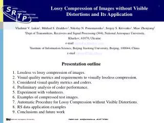
Vladimir V. Lukin1, Mikhail S. Zriakhov1, Nikolay N. Ponomarenko1, Sergey S. Krivenko1, Miao Zhenjiang2 1Dept of Transmitters, Receivers and Signal Processing (504), National Aerospace University, Kharkov, 61070, Ukraine e-mail lukin@ai.kharkov.com 2Institute of Information Science, Beijing Jiaotong University, Beijing, 100044, China e-mail zjmiao@bjtu.edu.cn Lossy Compression of Images without Visible Distortions and Its Application Presentation outline • Lossless vs lossy compression of images. • Visual quality metrics and requirements to visually lossless compression. • Considered visual quality metrics and coders. • Preliminary analysis of coder performance. • Experiment with volunteers. • Examples of compressed test images. • Automatic Procedure for Lossy Compression without Visible Distortions. • RS data application examples • Conclusions and future work Vladimir Lukin lukin@xai.kharkov.ua +38 057 7074841 Vladimir Lukin lukin@xai.kharkov.ua +38 057 7074841
Lossless compression: no losses are introduced but an attained compression ratio (CR) is often not appropriate for practice; Lossy compression: CR can be considerably larger (of the order of tens) but introduced losses can be not appropriate. In some applications it is thought that distortions due to lossy compression can lead to inevitable loss of useful (diagnostic, classification) information. Visually lossless (near-lossless, without visible distortions) compression can be a good trade-off for such applications and medical imaging, remote sensing, etc. A question is how to carry out visually lossless compression automatically with as high CR as possible? Lossless vs lossy compression of images Vladimir Lukin lukin@xai.kharkov.ua +38 057 7074841
For visually lossless compression, one needs: a quality metric able to adequately characterize visual quality of compressed images; a fixed threshold for which distortions are practically not seen irrespectively to a compressed image and a coder used; an automatic procedure for providing this threshold by an image compression method. There are quite many visual quality metrics nowadays but no one is perfect. For a particular application of image lossy compression, the metrics PSNR-HVS-M*, MSSIM** and some others produce quite good correspondence between these metrics and mean opinion score (MOS) for a large number of observers. *N. Ponomarenko, F. Silvestri, K. Egiazarian, M. Carli, J. Astola, V. Lukin, On between-coefficient contrast masking of DCT basis functions, CD-ROM Proceedings of the Third International Workshop on Video Processing and Quality Metrics, Scottsdale, USA, 4 p., January 2007. ** Wang Z., Simoncelli E.P., Bovik A.C., Multi-scale Structural Similarity for Visual Quality Assessment, Proceedings of the 37th IEEE Asilomar Conference on Signals, Systems and Computers, Vol. 2, pp. 1398-1402, 2003. Visual quality metrics and requirements to visually lossless compression Vladimir Lukin lukin@xai.kharkov.ua +38 057 7074841
Considered visual quality metrics: Standard PSNR, is expressed in dB, larger values correspond to better quality; this metric is widely used but is known to be not adequate to visual quality. PSNR-HVS-M (takes into account such peculiarities of human visual system (HVS) as lower sensitivity to distortions in high spatial frequency components and masking effects), is measured in dB, larger values correspond to better visual quality; the source code is freely available at www.ponomarenko.info; MSSIM (wavelet based, exploits multi-scale structural similarity of images), varies in the limits from 0 (very bad quality) to 1 (perfect quality). Considered visual quality metrics and coders Vladimir Lukin lukin@xai.kharkov.ua +38 057 7074841
Design of image quality measures that take into account HVS 5 Sample Distorted images PSNR = 21.06 dB PSNR = 21.06 dB PSNR = 21.39 dB PSNR-HVS = 29.09 dB PSNR-HVS = 37.78 dB PSNR-HVS = 18.98 dB Vladimir Lukin lukin@xai.kharkov.ua +38 057 7074841 29/09/2008
Analyzed coders The following lossy coders have been analyzed: • JPEG; • SPIHT (as available analog of JPEG2000); • AGU (performs in 32×32 pixel blocks, uses PPM coding of DCT coefficients, exploits deblocking at decompression stage); • ADCTC (is based on DCT, uses optimized partition schemes). HVS-oriented versions of AGU and ADCT coders (AGU-M and ADCTC-M, respectively) have been used. Example of partition scheme Vladimir Lukin lukin@xai.kharkov.ua +38 057 7074841
Preliminary analysis of coder performance Dependences of PSNR and PSNR-HVS-M vs CR for three coders for the test image Peppers PSNR-HVS-M is larger than PSNR (for medium CRs) due to taking into account masking effects. Vladimir Lukin lukin@xai.kharkov.ua +38 057 7074841
Preliminary analysis of coder performance Dependences of PSNR and PSNR-HVS-M vs CR for three coders for the test image Goldhill The same PSNR-HVS-M (e.g., 40 dB) is attained for different CR depending upon a coder and an image to be compressed. Vladimir Lukin lukin@xai.kharkov.ua +38 057 7074841
Preliminary analysis of coder performance Dependences of PSNR and PSNR-HVS-M vs CR for three coders for the test image Baboon PSNR-HVS-M is the largest for the coder ADCTC-M; for small CR PSNR-HVS-M for JPEG is larger than for SPIHT. Vladimir Lukin lukin@xai.kharkov.ua +38 057 7074841
Three test grayscale images (Baboon, Lena, and Goldhill) have been compressed with a large number of different CRs and, respectively, a large number and wide ranges of the values PSNR-HVS-M and MSSIM. For each compressed image, both PSNR-HVS-M and MSSIM have been determined. Compression has been done by several different coders including the standard JPEG, SPIHT, AGU, ADCTC, AGU-M, and ADCTC-M. Pairs of original and decompressed images have been simultaneously represented to each observer at monitor screen and observers had to decide are distortions visible or not. These decisions have been saved and processed in the following manner. For each subinterval of PSNR-HVS-M of width 1 dB (e.g., from 39 to 40 dB), all decisions (opinions) of all observers, all test images and all coders have been collected. Then, probabilities P of the fact that distortions are considered visible have been calculated for each subinterval. Experiments with volunteers (methodology) Vladimir Lukin lukin@xai.kharkov.ua +38 057 7074841
Experiments with volunteers (results) Table for PSNR, Probaility P for subintervals and different images Problem: for PSNR about 34.5 dB, about half of observers see difference between original and compressed images for simpler structure test images Peppers and Goldhill whilst in quarter of experiments people have noticed this difference for the textured image Baboon. Similarly, for PSNR about 31.5 dB, in about 89% of experiments difference between original and compressed images for simpler structure test images Peppers and Goldhill is seen whilst in half of experiments people have noticed this difference for the textured image Baboon. This makes problematic setting a fixed threshold of PSNR (or MSE) for providing visually lossless compression (although a practical recommendation could be 37 dB). Vladimir Lukin lukin@xai.kharkov.ua +38 057 7074841
Experiments with volunteers (results) Table for PSNR-HVS-M, Probaility P for subintervals and different images Main observation: the curves P vs PSNR-HVS-M for the three considered images are “closer” than the curves P vs PSNR. Averaged curves If P<0.2 is enough to consider that distortions are practically invisible, then it is possible to provide either PSNR-HVS-M not less than 40dB or MSSIM not less than 0.99. Vladimir Lukin lukin@xai.kharkov.ua +38 057 7074841
Examples of compressed test images QS=14.72, CR=9.16 PSNR-HVS-M=37.99 dB PSNR=27.36 dB MSSIM=0.9825 Original image Baboon, 512×512 pixels QS=12.21, CR=8.04 PSNR-HVS-M=39.92 dB PSNR=28.95 dB MSSIM=0.9859 Vladimir Lukin lukin@xai.kharkov.ua +38 057 7074841
Examples of compressed test images Original image Peppers, 512×512 pixels QS=12.79, CR=17.95 PSNR-HVS-M=39.98 dB PSNR=34.61 dB MSSIM=0.9851 QS=16.86, CR=22.37 PSNR-HVS-M=37.92 dB PSNR=33.99 dB MSSIM=0.9817 Vladimir Lukin lukin@xai.kharkov.ua +38 057 7074841
Therefore, a task is to provide lossy compression for a given full-reference metric Met of image visual quality and a given threshold Thr according to the following rule: If Met>Thr, then distortions are invisible and otherwise. (1) This should be done in automatic manner. Preliminary remarks: Control (variation) of CR is performed for different coders in different manner. For SPIHT and JPEG2000, this is done by setting a desired bpp (bits per pixel) where CR=8/bpp for standard 8-bit representation of grayscale images. For JPEG and other coders based on DCT, CR can be changed by varying quantization step (QS) in quantization tables. The solution is to apply iterative automatic procedure of multiple compression and decompression of a given image with estimation of controlled metric after each decompression and proper changing of a parameter that controls compression ratio. At the final stage, linear or spline approximation of rate/distortion curve is used to determine a final value of a parameter that controls CR. Then, the final lossy compression is performed with this determined value. Automatic Procedure for Lossy Compression without Visible Distortions Vladimir Lukin lukin@xai.kharkov.ua +38 057 7074841
Consider the plot of PSNR-HVS-M vs bpp for the test image Peppers. Suppose that at the first iteration step, compression and decompression have been done with bpp1=1. Also assume that we would like to provide PSNR-HVS-M approximately equal to 40 dB (with predetermined accuracy of, e.g., 0.3 dB which is appropriate for practical applications). Since we have original image and the image compressed/decompressed by SPIHT, it is possible to calculate PSNR-HVS-M1 for it. It occurs equal to 43.39 dB, i.e. larger than desired. Then, it is possible to take into consideration the fact that PSNR-HVS-M decreases if bpp reduces for any image. Thus, let us calculate bpp2 as bpp1- ∆bpp where ∆bpp denotes a step of changing the parameter that controls CR. At the second iteration, the original image is again subject to compression and decompression with bpp2. PSNR-HVS-M2 is determined and compared to the threshold (40 dB). If, at some i-th step, it occurs that PSNR-HVS-Mi<Thr and PSNR-HVS-Mi-1>Thr or PSNR-HVS-Mi>Thr and PSNR-HVS-Mi-1<Thr, a desired bppdes is between bppi-1 and bppi. Knowing PSNR-HVS-Mi, PSNR-HVS-Mi-1, Thr, bppi-1, and bppi, it is then easy to determine bppdes by approximation. The final compression is to be done with setting bppdes. Automatic Procedure for Lossy Compression without Visible Distortions (example) Vladimir Lukin lukin@xai.kharkov.ua +38 057 7074841
A middle-experience programmer can easily implement this algorithm. A number of iterations depends upon bpp1, ∆bpp and an image to be compressed. For 8-bit grayscale images we recommend to set bpp1=1.0 and ∆bpp=0.15, then for most images three or four iteration steps are enough. Similar automatic procedures are easily realizable for coders controlled by QS. Setting initial QS1=12 and the step ∆QS=2 allows providing a desired PSNR-HVS-M=40 dB in few iterations for most 8-bit grayscale images. The use of linear interpolation at the final stage for determination QSdes usually provides appropriate accuracy. The only thing one needs for starting the automatic procedure is to a priori know the character of a considered rate/distortion curve, i.e. is it monotonically increasing (as, e.g., PSNR-HVS-M on bpp) or decreasing (as, e.g., MSSIM on QS). Automatic Procedure for Lossy Compression without Visible Distortions (practical recommendations) Vladimir Lukin lukin@xai.kharkov.ua +38 057 7074841
Automatic Procedure for Lossy Compression without Visible Distortions Vladimir Lukin lukin@xai.kharkov.ua +38 057 7074841
Designed software Vladimir Lukin lukin@xai.kharkov.ua +38 057 7074841
The proposed approach to providing high visual quality of lossy image compression (without visible distortions) is useful for such applications where visual quality (but not larger compression ratio) is of prime importance. Till now, visual inspection of remote sensing data of different bands is widely used with different purposes. The proposed procedure has been applied component-wise to hyperspectral data obtained by AVIRIS and Hyperion imagers using AGU-M coder. CR for sub-band images of AVIRIS hyperspectral data is from 4 to 65, it depends upon complexity of a compressed sub-band image and signal-to-noise ratio in a given sub-band. CR values are, on the average, smaller for more complex images as Jasper Ridge and Moffett Field and larger for the images Lunar Lake and Cuprite. In aggregate, AGU-M coder provides total CR (for hypespectral data) of about 15 for Lunar Lake and Cuprite data and about 10 for Jasper Ridge and Moffett Field images, i.e. considerably larger than CR for the best lossless coders. Application examples (considered data and results) Vladimir Lukin lukin@xai.kharkov.ua +38 057 7074841
Application examples a) b) Image in 165-th sub-band of Lunar Lake AVIRIS before (а) and after (b) visually lossless compression, CR=5.0 (RAR provides CR=1.8, for ZIP archiver CR=1.6) Vladimir Lukin lukin@xai.kharkov.ua +38 057 7074841
Application examples a) b) Image in 224-th sub-band of Lunar Lake AVIRIS before (а) and after (b) visually lossless compression, CR=9.8 (RAR provides CR=2.5, for ZIP archiver CR=2.0) Vladimir Lukin lukin@xai.kharkov.ua +38 057 7074841
Application examples Dependence of CR on sub-band index 14-th sub-band of Hyperion image of Kiev Number of iterations Vladimir Lukin lukin@xai.kharkov.ua +38 057 7074841
The CR in sub-bands varied from 6 to 32 with aggregate CR approximately equal to 14. Thus, it is considerably larger than CR attained for lossless and near-lossless methods of hyperspectral image compression. QS used for compressing sub-band images varies in wide limits since dynamic range in sub-bands differs from each other. For each sub-band, it is approximately equal to that can be used as a starting point for iterative procedure. MSE of introduced distortions is of the order . CR values are smaller for sub-band images for which SNR is quite small. This deals with the fact that the coder “tries” to keep such images visually the same as originals and does not remove noise as lossy coders can do being applied to noisy images. Preliminary conclusions Vladimir Lukin lukin@xai.kharkov.ua +38 057 7074841
The automatic procedure for lossy image compression without visible distortions is proposed. Compression with MSSIM over 0.99 or PSNR-HVS-M over 40 dB should be provided for this purpose. Application examples for lossy compression of hyperspectral remote sensing data are given. In future, we plan to speed up iterative procedure of compression and to increase CR using 3D version of the coders (with grouping sub-band images). Conclusions and future work Vladimir Lukin lukin@xai.kharkov.ua +38 057 7074841