Download
1 / 9
90 likes | 176 Views
Learn to sketch a cycloid curve and its properties using symmetry and parametric equations. Explore the brachistochrone property of cycloids. Understand how to find tangent lines and slope on the curve.

E N D
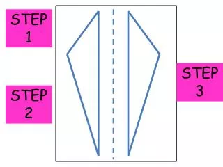
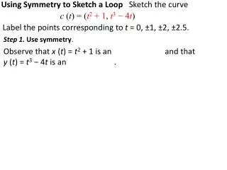
Using Symmetry to Sketch a Loop Sketch the curve c (t) = (t2 + 1, t3 − 4t) Label the points corresponding to t = 0, ±1, ±2, ±2.5. Step 1. Use symmetry. Observe that x (t) = t2 + 1 is an even function and that y(t) = t3 − 4t is an odd function. As noted before Example 5, this tells us that c (t) is symmetric with respect to the x-axis. Therefore, we will plot the curve for t ≥ 0 and reflect across the x-axis to obtain the part for t ≤ 0.
Using Symmetry to Sketch a Loop Sketch the curve c (t) = (t2 + 1, t3 − 4t) Label the points corresponding to t = 0, ±1, ±2, ±2.5. Step 2. Analyze x (t), y (t) as functions of t. We have x (t) = t2 + 1 and y (t) = t3 − 4t.
Using Symmetry to Sketch a Loop Sketch the curve c (t) = (t2 + 1, t3 − 4t) Label the points corresponding to t = 0, ±1, ±2, ±2.5. So the curve starts at c (0) = (1, 0), dips below the x-axis and returns to the x-axis at t = 2. Both x (t) and y (t) tend to ∞ as t→ ∞. The curve is concave up because y (t) increases more rapidly than x (t). Step 3. Plot points and join by an arc. The points c (0), c (1), c (2), c (2.5) are plotted and joined by an arc to create the sketch for t ≥ 0. The sketch is completed by reflecting across the x-axis.
A cycloid is a curve traced by a point on the circumference of a rolling wheel. Cycloids are famous for their “brachistochrone property”. A cycloid. A stellar cast of mathematicians (including Galileo, Pascal, Newton, Leibniz, Huygens, and Bernoulli) studied the cycloid and discovered many of its remarkable properties. A slide designed so that an object sliding down (without friction) reaches the bottom in the least time must have the shape of an inverted cycloid. This is the brachistochrone property, a term derived from the Greekbrachistos, “shortest,” andchronos, “time.”
Parametrizing the Cycloid Find parametric equations for the cycloid generated by a point P on the unit circle. The point P is located at the origin at t = 0. At time t, the circle has rolled t radians along the x axis and the center C of the circle then has coordinates (t, 1). Figure (B) shows that we get from C to P by moving down cost units and to the left sin t units, giving us the parametric equations
The argument on the last slide shows in a similar fashion that the cycloid generated by a circle of radius R has parametric equations
THEOREM 2 Slope of the Tangent Line Let c (t) = (x (t), y (t)), where x (t) and y (t) are differentiable. Assume that CAUTION Do not confuse dy/dx with the derivatives dx/dt and dy/dt, which are derivatives with respect to the parameter t. Only dy/dx is the slope of the tangent line.
Let c (t) = (t2 + 1, t3 − 4t). Find: (a) An equation of the tangent line at t = 3 (b) The points where the tangent is horizontal.