Download
1 / 21
210 likes | 362 Views
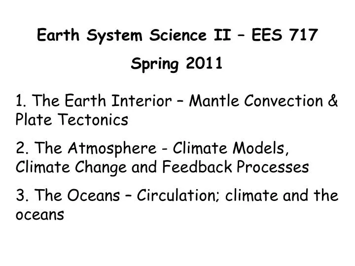
Earth System Science II – EES 717 Spring 2011 1. The Earth Interior – Mantle Convection & Plate Tectonics 2. The Atmosphere - Climate Models, Climate Change and Feedback Processes 3. The Oceans – Circulation; climate and the oceans.

E N D
Earth System Science II – EES 717 Spring 2011 1. The Earth Interior – Mantle Convection & Plate Tectonics 2. The Atmosphere - Climate Models, Climate Change and Feedback Processes 3. The Oceans – Circulation; climate and the oceans
Plate Tectonics is the surface expression of the mechanism by which heat escapes the Earth’s interior Onset of Thermal Boundary Layer Instability The fluid is initially at temperature T everywhere. Starting at time 0, the fluid is cooled from above, for example set Ttop = 0ºC. The top thermal boundary layer thickens with time. After a certain period of time, the thermal boundary layer becomes unstable as Rayleigh number characterizing the top boundary layer reaches a critical level. Cold downwellings develop from the thermal boundary layer, which limits the thickening of the boundary layer. The downwellings also cool the mantle.
And the forces are: F1: mantle drag – friction between the convecting asthenosphere and the overlying rigid lithosphere F2: gravitational ‘push’ – generated by high topography of MOR on the rest of oceanic plate F3: ‘pull’ on the opposite end of the plate into a subduction zone due to the increasing density of the oceanic lithosphere as it cools F4: the elastic resistance of the oceanic plate to being bent into a subduction zone F5: the tendency of the overriding plate to be drawn toward a subduction zone as the subducting slab bends (otherwise it would move away from the overriding plate) F6: friction between the subducting slab and the overlying lithosphere F7: tendency of the oceanic plate to sink as it cools and becomes denser (we can call that negative buoyancy)
A Primer on Convection • A system cooled from above or heated from within will develop an upper thermal boundary layer which drives the system. • The thermal boundary layer (plate, slab) is the only active element. • All upwellings are passive, and diffuse. • For large Prandtl number (the mantle) the mechanical boundary layers are the size of the mantle. • The scale of thermal boundary layers (plate thickness) is controlled by the Rayleigh number (Ra), which for the top is of the order of hundreds of km. • Ra is controlled both by physical properties (conductivity, expansivity etc.) and environment (heat flow, temperature gradients etc.).
A Primer on Convection • Both of these, physical factors and environment, cause Ra to be orders of magnitude lower at the base of mantle than at top. Therefore convective vigor is orders of magnitude less at the base of mantle. • The mechanical and thermal boundary layers at the base of mantle are therefore of the order of thousands of kilometers in lateral dimensions.
2. The Atmosphere • Things to review: • Atmospheric Composition and Structure • Heat Budget – Energy Transfer • Electromagnetic Radiation • The Greenhouse Effect • Feedbacks - Clouds • Global Circulation • ....
Focus: how reliable are the models used to make projections of future climate change? Global mean near-surface temperatures over the 20th century from observations (black) and as obtained from 58 simulations produced by 14 different climate models driven by both natural and human-caused factors that influence climate (yellow). The mean of all these runs is also shown (thick red line). Temperature anomalies are shown relative to the 1901 to 1950 mean. Vertical grey lines indicate the timing of major volcanic eruptions.
The projections of future climate change that these models make (IPCC, 2007): Multi-model averages and assessed ranges for surface warming at the end of the 21st century. Slines are multi-model global averages of surface warming (relative to 1980–1999) for the scenarios A2, A1B and B1, shown as continuations of the 20th century simulations. Shading denotes the ±1 standard deviation range of individual model annual averages. The orange line is for the experiment where concentrations were held constant at year 2000 values. The grey bars at right indicate the best estimate (solid line within each bar) and the likely range assessed for the six SRES marker scenarios. The assessment of the best estimate and likely ranges in the grey bars includes AOGCMs results as well as results from many independent models and observational constraints.
The projections of future climate change that these models make (IPCC, 2007): The table summarizes the projected global average surface warming and sea level rise at the end of the 21st century.
SW A*SW SW A*SW Review of Climate Feedbacks Water Vapor Feedback (+) Snow/ice – Albedo Feedback (+) IR flux – Temp. Feedback (–) Clouds Feedbacks ???????? Effects of Clouds on the Atmospheric Radiation Budget: SW radiation (top panel) and LW radiation (bottom panel)
Geostrophic gyres are gyres in balance between the pressure gradient and the Coriolis effect. Of the six great currents in the world’s ocean, five are geostrophic gyres. Note the western boundary currents in this map. 3. The Oceans
light color surface dark color deep 1. The Gulf Stream which transports heat from the tropics to northern Europe. 2. North Atlantic Deep Water formation which results from strong cooling. 3. Antarctic Bottom Water formation due to sea ice production around Antarctica.
Eddies: equivalent to atmospheric storms, ‘cascade’ of energy flow from large scale features down to the molecular level Mesoscale Eddies 50-200 km 1 – several months Geostrophic u = 0.1 m/s Ultimately the ocean’s kinetic energy is converted to heat, through frictional interaction with the sea-bed or internal friction at the molecular level (molecular visc.)
Kelvin Waves Travel eastward along the equator as a double wave ‘equatorial wave guide’ Travel along coasts (coast on right in the NH and on the left in the SH) Balance between pressure gradient force and coriolis force.
Rossby Waves: Propagate from east to west across basin Travel along lines of latitude Move slower than Kelvin waves Conservation of Potential Vorticity Example: Waves in the jet-stream
The Arctic Sea: Relatively enclosed basin (connection to the Pacific through the Bering Strait and to the Atlantic through the Greenland and Norwegian Seas) Enclosed nature influences ice cover Circulation: was originally deduced from ice flows and drifting ships, supplemented with direct current measurements and geostrophic calculations