Optimizing Investment and Resource Allocation for Project Management
100 likes | 211 Views
This guide focuses on using mathematical modeling to optimize investment decisions and resource allocation in project management. It addresses key concepts like Net Present Value (NPV) and cost constraints, while introducing variables that influence decision-making. The modeling framework highlights constraints related to project selection and resource limits, ensuring effective management of investment costs and potential profits. Examples include dishwashing product profitability and optimal ambulance deployment across cities, showcasing practical applications of mathematical models in business scenarios.

Optimizing Investment and Resource Allocation for Project Management
E N D
Presentation Transcript
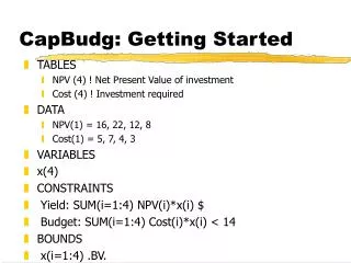
CapBudg: Getting Started • TABLES • NPV (4) ! Net Present Value of investment • Cost (4) ! Investment required • DATA • NPV(1) = 16, 22, 12, 8 • Cost(1) = 5, 7, 4, 3 • VARIABLES • x(4) • CONSTRAINTS • Yield: SUM(i=1:4) NPV(i)*x(i) $ • Budget: SUM(i=1:4) Cost(i)*x(i) < 14 • BOUNDS • x(i=1:4) .BV.
Other Constraints • Cannot invest in more than two projects • MaxProjects: SUM(i=1:4)x(i) < 2 • If we invest in project 2, we must invest in project 1 • If2Then1: x(2) < x(1) • If we invest in project 3, we cannot invest in project 4 • If3ThenNot4: x(3) + x(4) < 1 • If we invest in two projects, we must invest in project 1 • IfTwoThen1: SUM(i=2:4) x(i) < 1
Dish Wash: Fixed Charge • 3 Kinds of Dishwashers • Limited amounts of • Steel • Labor • If we make a product there’s a minimum quantity we can make economically • Otherwise, we don’t make the product • Maximize Profit
The Parameters (Tables) • LET NProd = 3 ! Number of products • TABLES • P(NProd) ! Unit profit • ST(NProd) ! Steel used per unit • STAVL ! Steel available • HR(NProd) ! Hours used per unit • HRAVL ! Hours available • UB(NProd) ! Upper bound on x - calculated • LB(NProd) ! Lower bound on x
The Model • ASSIGN • UB(p=1:NProd) = min(STAVL/ST(p), HRAVL/HR(p)) • VARIABLES • x(NProd) ! Amount of product made • mkx(NProd) ! 1 if any product made • CONSTRAINTS • Profit: SUM(p=1:NProd) P(p)*x(p) $ • SteelMax: SUM(p=1:NProd) ST(p)*x(p) < STAVL • HoursMax: SUM(p=1:NProd) HR(p)*x(p) < HRAVL • UBx(p=1:NProd): x(p) < UB(p)*mkx(p) • LBx(p=1:NProd): x(p) > LB(p)*mkx(p) • BOUNDS • mkx(p=1:NProd) .BV.
The Data • DATA • P = 25, 27, 35 • ST = 10, 13, 17 • STAVL = 90 • HR = 7, 5, 5 • HRAVL = 40 • LB = 2, 2.5, 2
Ambulance 2: Set Covering • 6 cities • Travel times between • Minimum number of ambulances so that one is within 20 minutes of every city
Parameters (TABLES) • LET NTown = 6 ! No. towns • LET TimeLimit = 20 ! Max time allowed to reach any town • TABLES • TIME(NTown,NTown) ! Time taken between each pair of towns • SERVE(NTown,NTown) ! 1 if time within limit, 0 otherwise
The Model • ASSIGN • SERVE(s=1:NTown,t=1:NTown) = & if (TIME(s,t) <= TimeLimit, 1, 0) • VARIABLES • open(NTown) ! 1 if ambulance at town; 0 if not • CONSTRAINTS • MinAmb: & Minimise number ambulances • SUM(t=1:NTown) open(t) $ • Serve(s=1:NTown): & Serve each town • SUM(t=1:NTown) SERVE(s,t) * open(t) > 1 • BOUNDS • open(t=1:NTown) .bv.
The Data • DATA • TIME(1,1) = 0,15,25,35,35,25 • TIME(2,1) = 15, 0,30,40,25,15 • TIME(3,1) = 25,30, 0,20,30,25 • TIME(4,1) = 35,40,20, 0,20,30 • TIME(5,1) = 35,25,35,20, 0,19 • TIME(6,1) = 25,15,25,30,19, 0