Download
1 / 21
230 likes | 452 Views
Contents of Chapter 7. Chapter 7 Backtracking 7.1 The General method 7.2 The 8-queens problem 7.3 Sum of subsets 7.4 Graph coloring 7.5 Hamiltonian cycles 7.6 Knapsack problem 7.7 References and readings 7.8 Additional exercises. 7.1 The General Method. Backtracking

E N D
Contents of Chapter 7 • Chapter 7 Backtracking • 7.1 The General method • 7.2 The 8-queens problem • 7.3 Sum of subsets • 7.4 Graph coloring • 7.5 Hamiltonian cycles • 7.6 Knapsack problem • 7.7 References and readings • 7.8 Additional exercises
7.1 The General Method • Backtracking • One of the most general techniques for searching a set of solutions or for searching an optimal solution • The name first coined by D.H. Lehmer • Basic idea of backtracking • Desired solution expressed as an n-tuple (x1,x2,…,xn) where xi are chosen from some set Si • If |Si|=mi, m=m1m2..mn candidates are possible • Brute force approach • Forming all candidates, evaluate each one, and saving the optimum one • Backtracking • Yielding the same answer with far fewer than m trials • “Its basic idea is to build up the solution vector one component at a time and to use modified criterion function Pi(x1,..,xi) (sometimes called bounding function) to test whether the vector being formed has any chance of success. The major advantage is: if it is realized that the partial vector (x1,..,xi) can in no way lead to an optimum solution, then mi+1…mn possible test vectors can be ignored entirely.”
7.1 The General Method • Constraints • Solutions must satisfy a set of constraints • Explicit vs. implicit • Definition 1: Explicit constraints are rules that restrict each xi to take on values only from a given set. • eg) xi 0 or Si = { all nonnegative real numbers } xi = 0 or 1 or Si = { 0, 1 } li xi ui or Si = {a : li a ui } • All tuples satisfying the explicit constraints define a possible solution space for I (I=problem instance) • Definition 2: The implicit constraints are rules that determine which of the tuples in the solution space of I satisfy the criterion function. Thus implicit constrains describe the way in which the xi must relate to each other.
7.1 The General Method • Example 7.1 (8-queens) • Classic combinatorial problem • Place eight queens on an 8*8 chessboard so that no two attack • Without loss of generality, assume that queen i is placed on row i • All solutions represented as 8-tuples (x1,x2,…,x8) where xi is the column on which queen i is placed • Constraints • Explicit constraints • Si={1,2,…,8} • So, solution space consists of 88 8-tuples • Implicit constraints • No two xi’s can be the same (By this, solution space reduced from 88 to 8!) • No two queens can be on the same diagonal
7.1 The General Method • Example 7.1 (Continued) • Figure 7.1 • 8-tuple = (4, 6, 8, 2, 7, 1, 3, 5)
7.1 The General Method • Example 7.2 (sum of subsets) • Given positive numbers wi, 1≤i≤n, and m, find all subsets of the wi whose sum is m • eg) (w1,w2,w3,w4) = (11,13,24,7) and m=31 • Solutions are (11,13,7) and (24,7) • Representation of solution vector • Variable-sized • By giving indices • In the above example, (1,2,4) and (3,4) • Explicit constraints: xi ∈ { j | j is integer and 1≤j≤n} • Implicit constraints: no two be the same, the sums are m • Fixed-sized • n-tuple (x1,x2,…,xn) where xi∈{0,1}, 1≤i≤n • In the above example, (1,1,0,1) and (0,0,1,1)
7.1 The General Method • Backtracking • Systematically searching the solution space by using a tree organization • Example 7.3 (n-queens) • Example of 4-queens problem (Figure 7.2) • 4!=24 leaf nodes
7.1 The General Method • Example 7.4 (sum of subsets) • Variable tuple size (Figure 7.3) • Solution space defined by all paths from the root to any node
7.1 The General Method • Example 7.4 (Continued) • Fixed tuple size (Figure 7.4) • Solution space defined by all paths from the root to a leaf node
7.1 The General Method • Terminology • The tree organization of the solution space is state space tree • Each node in the state space tree defines problem state • Solution state are those problem states s for which the path from the root to s defines a tuple in the solution space • eg) • In Figure 7.3, all nodes are solution state • In Figure 7.4, only leaf nodes are solution state • Answer state are those solution states s for which the path from root to s defines a tuple that is a member of solutions (it satisfies the implicit constraints) • Solution space is partitioned into disjoint sub-solution space at each internal node • Static vs. dynamic tree • Static trees are independent of the problem instance • Dynamic trees are dependent of the problem instance
7.1 The General Method • Terminology • A node which has been generated and all of whose children have not yet been generated is called a live node • The live node whose children are currently being generated is called E-node • A dead node is a generated node which is not to be expanded further or all of whose children have been generated • Two different ways of tree generation • Backtracking (Chapter 7) • Depth first node generation with bounding functions • Branch-and-bound (Chapter 8) • E-node remains E-node until it is dead
7.1 The General Method • Example 7.5 (4-queens) • This example shows how the backtracking works • Figure6 7.5
7.1 The General Method • Figure 7.6
void Backtrack( int k ) // This is a schema that describes the backtracking // process using recursion. On entering, the first k-1 // values x[1], x[2], …., x[k-1] of the solution vector // x[1:n] have been assigned. x[] and n are global. { for (each x[k] such that x[k] T(x[1], …, x[k-1]) { if (Bk (x[1], x[2], …, x[k])) { if (x[1], x[2], …, x[k] is a path to an answer node) output x[1:k]; if (k < n) Backtrack(k+1); } } } 7.1 The General Method • Formulation of the backtracking • T(x1,x2,…,xi): set of all possible values for xi+1 such that (x1,x2,…,xi,xi+1) is also a path to a problem state • Bi+1(x1,x2,…,xi,xi+1): bounding function • If Bi+1(x1,x2,…,xi,xi+1) is false, then the path cannot be extended to reach an answer node • Recursive backtracking algorithm (Program 7.1) • Initially invoked by Backtrack(1)
void IBacktrack( int n ) // This is a schema that describes the backtracking process. // All solutions are generated in x[1:n] and printed // as soon as they are determined. { int k=1; while (k) { if (there remains an untried x[k] such that x[k] is in T( x[1], x[2], …, x[k-1] ) and Bk(x[1], …,x[k]) is true) { if ( x[1], …, x[k] is a path to an answer node ) output x[1:k]; k++; // Consider the next set. } else k--; // Backtrack to the previous set. } } 7.1 The General Method • Iterative backtracking algorithm (Program 7.2)
7.1 The General Method • Four factors for efficiency of the backtracking algorithms • Time to generate the next xk • Number of xk satisfying the explicit constraints • Time for the bounding function Bk • Number of xk satisfying Bk * The first three relatively independent of the problem instance, and the last dependent
bool Place(int k, int i) // Returns true if a queen can be placed in kth row and // ith column. Otherwise it returns false. x[] is a // global array whose first (k-1) values have been set. // abs(r) returns the absolute value of r. { for (int j=1; j < k; j++) if ((x[j] == i) // Two in the same column || (abs(x[j]-i) == abs(j-k))) // or in the same diagonal return(false); return(true); } 7.2 The 8-Queens Problem • Bounding function • No two queens placed on the same column xi’s are distinct • No two queens placed on the same diagonal how to test? • The same value of “row-column” or “row+column” • Supposing two queens on (i,j) and (k,l) • i-j=k-l (i.e., j-l=i-k) or i+j=k+l (i.e., j-l=k-i) • So, two queens placed on the same diagonal iff |j-l| = |i-k| • Bounding function: can a new queen be placed ? (Program 7.4)
void NQueens(int k, int n) // Using backtracking, this procedure prints all // possible placements of n queens on an nXn // chessboard so that they are nonattacking. { for (int i=1; i<=n; i++) { if (Place(k, i)) { x[k] = i; if (k==n) { for (int j=1;j<=n;j++) cout << x[j] << ' '; cout << endl;} else NQueens(k+1, n); } } } 7.2 The 8-Queens Problem • Backtracking algorithm for the n-queens problem (Program 7.5) • Invoked by Nqueens(1,n)
7.3 Sum of Subsets • Bounding function • Bk(x1,..,xk)=true iff • Assuming wi’s in nondecreasing order, (x1,..,xk) cannot lead to an answer node if • So, the bounding function is
7.3 Sum of Subsets • Backtracking algorithm for the sum of sunsets (Program 7.6) • Invoked by SumOfSubsets(0,1,∑i=1,nwi) void SumOfSub(float s, int k, float r) // Find all subsets of w[1:n] that sum to m. The values // of x[j], 1<=j<k, have already been determined. // s= ∑j=1,k-1 w[j]*x[j] and r= ∑j=k,nw[j]. // The w[j]'s are in nondecreasing order. // It is assumed that w[1]<=m and ∑i=1n w[i]>=m. { // Generate left child. Note that s+w[k] <= m // because Bk-1 is true. x[k] = 1; if (s+w[k] == m) { // Subset found for (int j=1; j<=k; j++) cout << x[j] << ' '; cout << endl; } // There is no recursive call here as w[j] > 0, 1 <= j <= n. else if (s+w[k]+w[k+1] <= m) SumOfSub(s+w[k], k+1, r-w[k]); // Generate right child and evaluate Bk-1. if ((s+r-w[k] >= m) && (s+w[k+1] <= m)) { x[k] = 0; SumOfSub(s, k+1, r-w[k]); } }
7.3 Sum of Subsets • Example 7.6 (Figure 7.10) • n=6, w[1:6]={5,10,12,13,15,18}, m=30