Download
1 / 34
360 likes | 858 Views
Contents of Chapter 4. Chapter 4 The Greedy method 4.1 The general method 4.2 Knapsack problem 4.3 Tree vertex splitting 4.4 Job sequencing with deadlines 4.5 Minimum cost spanning trees 4.6 Optimal storage on tapes 4.7 Optimal merge patterns 4.8 Single-source shortest paths

E N D
Contents of Chapter 4 • Chapter 4 The Greedy method • 4.1 The general method • 4.2 Knapsack problem • 4.3 Tree vertex splitting • 4.4 Job sequencing with deadlines • 4.5 Minimum cost spanning trees • 4.6 Optimal storage on tapes • 4.7 Optimal merge patterns • 4.8 Single-source shortest paths • 4.9 References and readings • 4.10 Additional exercises
SolType Greedy(Type a[], int n) // a[1:n] contains the n inputs. { SolType solution = EMPTY; // Initialize the solution for (int i = 1; i <= n; i++) { Type x = Select(a); if Feasible(solution, x) solution = Union(solution, x); } return solution; } 4.1 General Method • Greedy method control abstraction for subset paradigm (Program 4.1) • Terminologies: feasible solution, objective function, optimal solution • Subset paradigm vs. ordering paradigm • Subset paradigm: selection of optimal subset (Sec. 4.2 – 4.5) • Ordering paradigm: finding optimal ordering (Sec. 4.6-4.8)
4.2 Knapsack Problem • Problem definition • Given n objects and a knapsack where object i has a weight wi and the knapsack has a capacity m • If a fraction xi of object i placed into knapsack, a profit pixi is earned • The objective is to obtain a filling of knapsack maximizing the total profit • Problem formulation (Formula 4.1-4.3) • A feasible solution is any set satisfying (4.2) and (4.3) • An optimal solution is a feasible solution for which (4.1) is maximized
4.2 Knapsack Problem • Example 4.1 • n=3, m=20, (p1,p2,p3)=(25,24,15), (w1,w2,w3)=(18,15,10) 1. (1/2, 1/3, 1/4) 16.5 24.25 2. (1, 2/15, 0) 20 28.2 3. (0, 2/3, 1) 20 31 4. (0, 1, 1/2) 20 31.5 • Lemma 4.1 In case the sum of all the weights is ≤ m, then xi = 1, 1 ≤ i ≤ n is an optimal solution. • Lemma 4.2 All optimal solutions will fill the knapsack exactly. • Knapsack problem fits the subset paradigm
4.2 Knapsack Problem • Greedy strategy using total profit as optimization function • Solution 2 in Example 4.1 • Suboptimal • Greedy strategy using weight (capacityused) as optimization function • Solution 3 in Example 4.1 • Suboptimal • Greedy strategy using ratio of profit to weight (pi/wi) as optimization function • Solution 4 in Example 4.1 • Optimal
void GreedyKnapsack(float m, int n) // p[1:n] and w[1:n] contain the profits and weights // respectively of the n objects ordered such that // p[i]/w[i] >= p[i+1]/w[i+1]. m is the knapsack // size and x[1:n] is the solution vector. { for (int i=1; i<=n; i++) x[i] = 0.0; // Initialize x. float U = m; for (i=1; i<=n; i++) { if (w[i] > U) break; x[i] = 1.0; U -= w[i]; } if (i <= n) x[i] = U/w[i]; } 4.2 Knapsack Problem • Algorithm for greedy strategies (Program 4.2) • Assuming the objects already sorted into nonincreasing order of pi/wi
4.2 Knapsack Problem • Time complexity • Sorting: O(n log n) using fast sorting algorithm like merge sort • GreedyKnapsack: O(n) • So, total time is O(n log n) • Theorem 4.1 If p1/w1 ≥ p2/w2 ≥ … ≥ pn/wn, then GreedyKnapsack generates an optimal solution to the given instance of the knapsack problem. • Proving technique Compare the greedy solution with any optimal solution. If the two solutions differ, then find the first xi at which they differ. Next, it is shown how to make the xi in the optimal solution equal to that in the greedy solution without any loss in total value. Repeated use of this transformation shows that the greedy solution is optimal.
4.4 Job Sequencing with Deadlines • Example 4.2 • n=4, (p1,p2,p3,p4)=(100,10,15,27), (d1,d2,d3,d4)=(2,1,2,1) Feasible processing Solution sequence value 1. (1, 2) 2, 1 110 2. (1, 3) 1, 3 or 3, 1 115 3. (1, 4) 4, 1 127 4. (2, 3) 2, 3 25 5. (3, 4) 4, 3 42 6. (1) 1 100 7. (2) 2 10 8. (3) 3 15 9. (4) 4 27
4.4 Job Sequencing with Deadlines • Greedy strategy using total profit as optimization function • Applying to Example 4.2 • Begin with J= • Job 1 considered, and added to J J={1} • Job 4 considered, and added to J J={1,4} • Job 3 considered, but discarded because not feasible J={1,4} • Job 2 considered, but discarded because not feasible J={1,4} • Final solution is J={1,4} with total profit 127 • It is optimal • How to determine the feasibility of J ? • Trying out all the permutations • Computational explosion since there are n! permutations • Possible by checking only one permutation • By Theorem 4.3 • Theorem 4.3 Let J be a set of k jobs and a permutation of jobs in J such that Then J is a feasible solution iff the jobs in J can be processed in the order without violating any deadline.
4.4 Job Sequencing with Deadlines • Theorem 4.4 The greedy method described above always obtains an optimal solution to the job sequencing problem. • High level description of job sequencing algorithm (Program 4.5) • Assuming the jobs are ordered such that p[1]p[2]…p[n] GreedyJob(int a[], set J, int n) // J is a set of jobs that can be // completed by their deadlines. { J = {1}; for (int i=2; i<=n; i++) { if (all jobs in J ∪{i} can be completed by their deadlines) J = J ∪{i}; } }
4.4 Job Sequencing with Deadlines • How to implement Program 4.5 ? • How to represent J to avoid sorting the jobs in J each time ? • 1-D array J[1:k] such that J[r], 1rk, are the jobs in J and d[J[1]] d[J[2]] …. d[J[k]] • To test whether J {i} is feasible, just insert i into J preserving the deadline ordering and then verify that d[J[r]]r, 1rk+1
4.4 Job Sequencing with Deadlines • C++ description of job sequencing algorithm (Program 4.6) int JS(int d[], int j[], int n) // d[i]>=1, 1<=i<=n are the deadlines, n>=1. The jobs // are ordered such that p[1]>=p[2]>= ... >=p[n]. J[i] // is the ith job in the optimal solution, 1<=i<=k. // Also, at termination d[J[i]]<=d[J[i+1]], 1<=i<k. { d[0] = J[0] = 0; // Initialize. J[1] = 1; // Include job 1. int k=1; for (int i=2; i<=n; i++) { //Consider jobs in nonincreasing // order of p[i]. Find position for // i and check feasibility of insertion. int r = k; while ((d[J[r]] > d[i]) && (d[J[r]] != r)) r--; if ((d[J[r]] <= d[i]) && (d[i] > r)) { // Insert i into J[]. for (int q=k; q>=(r+1); q--) J[q+1] = J[q]; J[r+1] = i; k++; } } return (k); }
4.5 Minimum-cost Spanning Trees • Definition 4.1 Let G=(V, E) be at undirected connected graph. A subgraph t=(V, E’) of G is a spanning tree of G iff t is a tree. • Example 4.5 • Applications • Obtaining an independent set of circuit equations for an electric network • etc Spanning trees
4.5 Minimum-cost Spanning Trees • Example of MCST (Figure 4.6) • Finding a spanning tree of G with minimum cost 1 1 28 2 2 10 10 16 16 14 14 3 3 6 7 6 7 24 25 18 25 12 12 5 5 4 4 22 22 (a) (b)
4.5.1 Prim’s Algorithm • Example 4.6 (Figure 4.7) 1 1 1 10 10 10 2 2 2 3 3 3 6 7 7 6 7 6 25 25 5 5 5 4 4 4 22 (a) (b) (c) 1 1 1 10 10 10 2 2 2 16 16 14 3 3 7 6 3 7 6 7 6 25 25 12 25 12 12 5 5 5 4 22 4 22 4 22 (d) (e) (f)
4.5.1 Prim’s Algorithm • Implementation of Prim’s algorithm • How to determine the next edge to be added? • Associating with each vertex j not yet included in the tree a value near(j) • near(j): a vertex in the tree such that cost(j,near(j)) is minimum among all choices for near(j) • The next edge is defined by the vertex j such that near(j)0 (j not already in the tree) and cost(j,near(j)) is minimum • eg, Figure 4.7 (b) near(1)=0 // already in the tree near(2)=1, cost(2, near(2))=28 near(3)=1 (or 5 or 6), cost(3, near(3))= // no edge to the tree near(4)=5, cost(4, near(4))=22 near(5)=0 // already in the tree near(6)=0 // already in the tree near(7)=5, cost(7, near(7))=24 So, the next vertex is 4
4.5.1 Prim’s Algorithm • Prim’s MCST algorithm (Program 4.8) 1 float Prim(int E[][SIZE], float cost[][SIZE], int n, int t[][2]) 11 { 12 int near[SIZE], j, k, L; 13 let (k,L) be an edge of minimum cost in E; 14 float mincost = cost[k][L]; 15 t[1][1] = k; t[1][2] = L; 16 for (int i=1; i<=n; i++) // Initialize near. 17 if (cost[i][L] < cost[i][k]) near[i] = L; 18 else near[i] = k; 19 near[k] = near[L] = 0; 20 for (i=2; i <= n-1; i++) { // Find n-2 additional 21 // edges for t. 22 let j be an index such that near[j]!=0 and 23 cost[j][near[j]] is minimum; 24 t[i][1] = j; t[i][2] = near[j]; 25 mincost = mincost + cost[j][near[j]]; 26 near[j]=0; 27 for (k=1; k<=n; k++) // Update near[]. 28 if ((near[k]!=0) && 29 (cost[k][near[k]]>cost[k][j])) 30 near[k] = j; 31 } 32 return(mincost); 33 }
4.5.1 Prim’s Algorithm • Time complexity • Line 13: O(|E|) • Line 14: (1) • for loop of line 16: (n) • Total of for loop of line 20: O(n2) • n iterations • Each iteration • Lines 22 & 23: O(n) • for loop of line 27: O(n) • So, Prim’s algorithm: O(n2) • More efficient implementation using red-black tree • Using red-black tree • Lines 22 and 23 take O(log n) • Line 27: O(|E|) • So total time: O((n+|E|) log n)
4.5.2 Kruskal’s Algorithm • Example 4.7 (Figure 4.8) 1 1 1 10 10 2 2 2 3 3 3 7 7 6 7 6 6 12 5 5 5 4 4 4 (a) (b) (c) 1 1 1 10 10 2 10 2 2 14 16 14 14 16 3 3 6 7 3 6 7 6 7 12 12 12 5 5 5 4 22 4 4 (d) (e) (f)
4.5.2 Kruskal’s Algorithm • Pseudo code of Kruskal’s algorithm (Program 4.9) • How to implement ? • Two functions should be considered • Determining an edge with minimum cost (line 3) • Deleting this edge (line 4) • Using minheap • Construction of minheap: O(|E|) • Next edge processing: O(log |E|) • Using Union/Find set operations to maintain the intermediate forest t = EMPTY; while ((t has fewer than n-1 edges) && (E!=EMPTY)) { choose an edge (v, w) from E of lowest cost;; delete (v, w) from E; if (v, w) dose not create a cycle in t add (v, w) to t; else discard (v, w); }
4.5.2 Kruskal’s Algorithm • Kruskal’s algorithm (Program 4.10) float Kruskal(int E[][SIZE], float cost[][SIZE], int n, int t[][2]) { int parent[SIZE]; construct a heap out of the edge costs using Heapify; for (int i=1; i<=n; i++) parent[i] = -1; // Each vertex is in a different set. i = 0; float mincost = 0.0; while ((i < n-1) && (heap not empty)) { delete a minimum cost edge (u,v) from the heap and reheapify using Adjust; int j = Find(u); int k = Find(v); if (j != k) { i++; t[i][1] = u; y[i][2] = v; mincost += cost[u][v]; Union(j, k); } } if ( i != n-1) cout << “No spanning tree” << endl; else return(mincost); }
4.7 Optimal Merge Patterns • Problem • Given n sorted files, find an optimal way (i.e., requiring the fewest comparisons or record moves) to pairwise merge them into one sorted file • It fits ordering paradigm • Example 4.9 • Three sorted files (x1,x2,x3) with lengths (30, 20, 10) • Solution 1: merging x1 and x2 (50 record moves), merging the result with x3 (60 moves) total 110 moves • Solution 2: merging x2 and x3 (30 moves), merging the result with x1 (60 moves) total 90 moves • The solution 2 is better
z4 95 z2 35 60 z3 z1 15 20 30 30 x5 x2 x1 5 10 x4 x3 4.7 Optimal Merge Patterns • A greedy method (for 2-way merge problem) • At each step, merge the two smallest files • e.g., five files with lengths (20,30,10,5,30) (Figure 4.11) • Total number of record moves = weighted external path length • The optimal 2-way merge pattern = binary merge tree with minimum weighted external path length
4.7 Optimal Merge Patterns • Algorithm (Program 4.13) struct treenode { struct treenode *lchild, *rchild; int weight; }; typedef struct treenode Type; Type *Tree(int n) // list is a global list of n single node // binary trees as described above. { for (int i=1; i<n; i++) { Type *pt = new Type; // Get a new tree node. pt -> lchild = Least(list); // Merge two trees with pt -> rchild = Least(list); // smallest lengths. pt -> weight = (pt->lchild)->weight + (pt->rchild)->weight; Insert(list, *pt); } return (Least(list)); // Tree left in l is the merge tree. }
4.7 Optimal Merge Patterns • Example 4.10 (Figure 4.12)
4.7 Optimal Merge Patterns • Time • If list is kept in nondecreasing order: O(n2) • If list is represented as a minheap: O(n log n)
0 1 M4 0 1 M3 1 0 M1 M2 4.7 Optimal Merge Patterns • Huffman codes • Obtaining an optimal set of codes for messages M1, M2, .., Mn+1 • e.g, 4 messages (Figure 4.14) • M1=000 • M2=001 • M3=01 • M4=1
4.7 Optimal Merge Patterns • Huffman codes (Continued) • When qi is the relative frequency for Mi • The expected decode time (also the expected message length) • The minimum decode time (also minimum message length) is possible by choosing the code words resulting in a binary tree with minimum weighted external path length (that is, the same algorithm as 2-way merge problem is applicable) • Example using Exercise 4 • (q1,q2,…,q7)=(4,5,7,8,10,12,20)
4.8 Single-source Shortest Paths • Example 4.11 (Figure 4.15)
4.8 Single-source Shortest Paths • Design of greedy algorithm • Building the shortest paths one by one, in nondecreasing order of path lengths • e.g., in Figure 4.15 • 14: 10 • 145: 25 • … • We need to determine 1) the next vertex to which a shortest path must be generated and 2) a shortest path to this vertex • Notations • S = set of vertices (including v0 ) to which the shortest paths have already been generated • dist(w) = length of shortest path starting from v0, going through only those vertices that are in S, and ending at w
4.8 Single-source Shortest Paths • Design of greedy algorithm (Continued) • Three observations • If the next shortest path is to vertex u, then the path begins at v0, ends at u, and goes through only those vertices that are in S. • The destination of the next path generated must be that of vertex u which has the minimum distance, dist(u), among all vertices not in S. • Having selected a vertex u as in observation 2 and generated the shortest v0 to u path, vertex u becomes a member of S.
ShortestPaths(int v, float cost[][SIZE], float dist[], int n) { int u; bool S[SIZE]; for (int i=1; i<= n; i++) { // Initialize S. S[i] = false; dist[i] = cost[v][i]; } S[v]=true; dist[v]=0.0; // Put v in S. for (int num = 2; num < n; num++) { // Determine n-1 paths from v. choose u from among those vertices not in S such that dist[u] is minimum; S[u] = true; // Put u in S. for (int w=1; w<=n; w++) //Update distances. if (( S[w]=false) && (dist[w] > dist[u] + cost[u][w])) dist[w] = dist[u] + cost[u][w]; } } 4.8 Single-source Shortest Paths • Greedy algorithm (Program 4.14): Dijkstra’s algorithm • Time: O(n2)
4.8 Single-source Shortest Paths • Example 4.12 (Figures 4.16)
4.8 Single-source Shortest Paths • Example 4.12 (Figures 4.17)