Download
1 / 59
590 likes | 684 Views
Contextual models for object detection using boosted random fields. by Antonio Torralba, Kevin P. Murphy and William T. Freeman. Quick Introduction. What is this? Now can you tell?. Belief Propagation (BP). Network (Pairwise Markov Random Fields) observed nodes ( y i ).

E N D
Contextual models for object detection using boosted random fields by Antonio Torralba, Kevin P. Murphy and William T. Freeman
Quick Introduction • What is this? • Now can you tell?
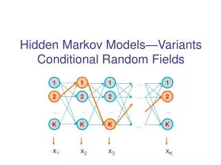
Belief Propagation (BP) • Network (Pairwise Markov Random Fields) • observed nodes (yi)
Belief Propagation (BP) • Network (Pairwise Markov Random Fields) • observed nodes (yi) • hidden nodes (xi)
Belief Propagation (BP) • Network (Pairwise Markov Random Fields) • observed nodes (yi) • hidden nodes (xi) Statistical dependency, called local evidence: Shord-hand
Belief Propagation (BP) Statistical dependency: Local evidence Shord-hand Statistical dependency: Compatibility function
Belief Propagation (BP) • Joint probability
Belief Propagation (BP) • Joint probability x x1 x2 y1 y2 xi …. yi x5 x3 x1 x4 x12 xj
Belief Propagation (BP) • Joint probability x x1 x2 y1 y2 xi …. yi x5 x3 x1 x4 x12 xj
Belief Propagation (BP) • The belief b at a node i is represented by • the local evidence of the node • all the messages coming in from neighbors Ni xi xj ∏ yi
Belief Propagation (BP) • The belief b at a node i is represented by • the local evidence of the node • all the messages coming in from neighbors Ni xi xj ∏ yi
Belief Propagation (BP) • Messages m between hidden nodes • How likely node j thinks it is that node i will be in the corresponding state. mji(xi) xi xj
Belief Propagation (BP) mji(xi) xi xj xi xj xk
Conditional Random Field • Distribution of the form:
Conditional Random Field • Distribution of the form:
Boosted Random Field • Basic Idea: • Use BP to estimate P(x|y) • Use boosting to maximize Log Likelihood of each node wrt to
Algorithm: BP • Minimize negative log likelihood of training data (yi). Label Loss function to minimize:
Algorithm: BP • Minimize negative log likelihood of training data (yi). Label Loss function to minimize:
Algorithm: BP • Minimize negative log likelihood of training data (yi). Label Loss function to minimize:
Algorithm: BP Ni xi xj ∏ yi
Algorithm: BP Ni xi xj ∏ yi
Algorithm: BP Ni xi xj ∏
Algorithm: BP xi xj
Algorithm: BP xi yi F: a function of the input data
Algorithm: BP yi xj xi with
Algorithm: BP yi xj xi with
Function F yi • Boosting! • f is the weak learner:weighted decision stumps. xi
Minimization of loss L where
Local Evidence: algorithm yi • For t=1..T • Iterate Nboost times • find the best basis function h • update local evidence with • update the beliefs • update the weights • Iterate NBP times • update messages • update the beliefs xj xi
Local Evidence: algorithm yi • For t=1..T • Iterate Nboost times • find the best basis function h • update local evidence with • update the beliefs • update the weights • Iterate NBP times • update messages • update the beliefs xj xi
Local Evidence: algorithm yi • For t=1..T • Iterate Nboost times • find the best basis function h • update local evidence with • update the beliefs • update the weights • Iterate NBP times • update messages • update the beliefs xj xi
Local Evidence: algorithm yi • For t=1..T • Iterate Nboost times • find the best basis function h • update local evidence with • update the beliefs • update the weights • Iterate NBP times • update messages • update the beliefs xj xi
Local Evidence: algorithm yi • For t=1..T • Iterate Nboost times • find the best basis function h • update local evidence with • update the beliefs • update the weights • Iterate NBP times • update messages • update the beliefs xj xi
Local Evidence: algorithm yi • For t=1..T • Iterate Nboost times • find the best basis function h • update local evidence with • update the beliefs • update the weights • Iterate NBP times • update messages • update the beliefs xj xi
Function G • By assuming that the graph is densely connected we can make the approximation: • Now G is a non-linear additive function of the beliefs:
Function G • Instead of learning the function can be learnt with an additive model: weighted regression stumps
Function G • The weak learner is chosen by minimizing the loss:
The Boosted Random Field Algorithm • For t=1..T • find the best basis function h for f • find the best basis function for • compute local evidence • compute compatibilities • update the beliefs • update weights xj xi yi
The Boosted Random Field Algorithm • For t=1..T • find the best basis function h forf • find the best basis function for • compute local evidence • compute compatibilities • update the beliefs • update weights b1 xi b2 … bj
Final classifier • For t=1..T • update local evidences F • update compatibilities G • compute current beliefs • Output classification:
Multiclass Detection • U: Dictionary of ~2000 images patches • V: Same number of image masks
Multiclass Detection • U: Dictionary of ~2000 images patches • V: Same number of image masks • At each round t, for each class c for each dictionary entry d there is a weak learner:
Function f • To take into account different sizes, we first downsample the image and then upsample and OR the scales: • which is our function for computing the local evidence.
Function g • The compatibily function has a similar form:
Function g • The compatibily function has a similar form: • W represent a kernel with all the messages directed to node x,y,c
Kernels W • Example of incoming messages:
Function G • The overall incoming messages function is given by:
Learning… • Labeled dataset of office and street scenes, with each ~100 images • In the first 5 round updated only the local evidence • After the 5th iteration update also the compatibility functions • At each round update onlyF and G of the single object class that reduces the most the multiclass cost.