Classical Probabilistic Models and Conditional Random Fields
Classical Probabilistic Models and Conditional Random Fields. Roman Klinger 1 , Katrin Tomanek 2 Algorithm Engineering Report (TR07-2-013), 2007 1. Dortmund University of Technology Department of Computer Science 2. Language & Information Engineering (JULIE) Lab. Abstract. Introduction

Classical Probabilistic Models and Conditional Random Fields
E N D
Presentation Transcript
Classical Probabilistic Models and Conditional Random Fields Roman Klinger1, Katrin Tomanek2 Algorithm Engineering Report (TR07-2-013), 2007 1. Dortmund University of Technology Department of Computer Science 2. Language & Information Engineering (JULIE) Lab
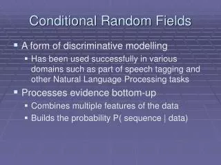
Abstract • Introduction • Naïve Bayes • HMM • ME • CRF
Introduction • Classification is known as the assignment of a class y ∈ Y to an observation x ∈ X • A well-known example (Russell and Norvig, 2003) • Classification of weather • Y = {good, bad} • X = {Monday, Tuesday,…} • x can be described by a set of features • fcloudy, fsunny or frainy In general, not necessary have to be binary
Modeling all dependenciesin a probability distribution is typically very complex due to interdependencies between features • The Naïve Bayes assumption of all features being conditionally independent is an approach to address this problem • In nearly all probabilistic models such independence assumptions are made for some variables to make necessary computations manageable
In the structured learning scenario, multiple and typically interdependent class and observation variables are considered which implicates an even higher complexity in the probability distribution • As for images, pixels near to each other are very likely to have a similar color or hue • In music, different succeeding notes follow special laws, they are not independent, especially when they sound simultaneously. Otherwise, music would not be pleasant to the ear • In text, words are not an arbitrary accumulation, the order is important and grammatical constraints hold
Y = {name, city, 0} X: set of words
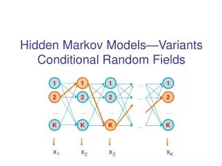
One approach for modeling linear sequence structures, as can be found in natural language text, are HMMs • For the sake of complexity reduction, strong independence assumptions between the observation variables are made • This impairs the accuracy of the model observation variables
Conditional Random Fields (CRFs, Lafferty et al. (2001)) are developed exactly to fill that gap: • While CRFs make similar assumptions on the dependencies among the class variables, no assumptions on the dependencies among observation variables need to be made observation variables
In natural language processing, CRFs are currently a state-of-the-art technique for many of its subtasks including • basic text segmentation (Tomanek et al., 2007) • part-of-speech tagging (Lafferty et al., 2001) • shallow parsing (Sha and Pereira, 2003) • the resolution of elliptical noun phrases (Buyko et al., 2007) • named entity recognition (Settles, 2004; McDonald and Pereira, 2005; Klinger et al., 2007a,b; McDonald et al., • 2004) • gene prediction (DeCaprio et al., 2007) • image labeling (He et al., 2004) • object recognition (Quattoni et al., 2005) • telematics for intrusion detection (Gupta et al., 2007) • sensor data management (Zhang et al., 2007)
Abstract • Introduction • Naïve Bayes • HMM • ME • CRF
Naïve Bayes • A conditional probability model is a probability distribution with an input vector , where are features and is the class variable to be predicted. That probability can be formulated with Bayes' law • : tag • : word (1) not used here
constant for all y Complex: Model probabilities conditioned on various # of variables (2) 1 2 3 (3)
In practice, it is often assumed, that all input variables are conditionally independent of each other which is known as the Naïve Bayes assumption
Simple: Model probabilities conditioned on only y (4) less complex than (3)
Dependencies between the input variables are not modeled, probably leading to an imperfect representation of the real world • Nevertheless, the Naïve Bayes Model performs surprisingly well in many real world applications, such as email classification (Androutsopoulos et al., 2000a,b; Kiritchenko and Matwin, 2001)
Abstract • Introduction • Naïve Bayes • HMM • ME • CRF
HMM • In the Naïve Bayes Model, only single output variables have been considered • To predict a sequence of class variables for an observation sequence a simple sequence model can be formulated as a product over single Naïve Bayes Models
Note, that in contrast to the Naïve Bayes Model there is only one feature at each sequenceposition, namely the identity of the respective observation • Dependencies between single sequence positions are not taken into account • Each observation xi depends only on the class variable yi at the respective sequence position (5) X X Naïve Bayes
it is reasonable to assume that there are dependencies between the observations at consecutive sequence positions (5) (6) (7)
Dependencies between output variables~y are modeled. A shortcoming is the assumption of conditional independence (see equation 6) between the input variables~x due to complexity issues • As we will see later, CRFs address exactly this problem
Abstract • Introduction • Naïve Bayes • HMM • ME • CRF
ME (Maximum Entropy) • The previous two models are trained to maximize the joint likelihood • In the following, the Maximum Entropy Model is discussed in more detail as it is fundamentally related to CRFs
The Maximum Entropy Model is a conditional probability model • It is based on the Principle of Maximum Entropy (Jaynes, 1957) which states that if incomplete information about a probability distribution is available, the only unbiased assumption that can be made is a distribution which is as uniform as possible given the available information
Under this assumption, the proper probability distribution is the one which maximizes the entropy given the constraints from the training material • For the conditional model p(y|x) the conditional entropy H(y|x) (Korn and Korn, 2000; Bishop, 2006) is applied, which is defined as (8)
The basic idea behind Maximum Entropy Models is to find the model p*(y|x) which on the one hand has the largest possible conditional entropy but is on the other hand still consistent with the information from the training material • The objective function, later referred to as primal problem, is thus (9)
The training material is represented by features • Here, these are defined as binary-valued functions which depend on both the input variable x and the class variable y. An example for such a function is (10)
The expected value of each featurefi is estimated from the empirical distribution ~ p(x; y) • The empirical distribution is obtained by simply counting how often the different values of the variables occur in the training data (11)
(11) • As the empirical probability for a pair (x, y) which is not contained in the training material is 0 • can be rewritten as • The size of the training set is • can be calculated by counting how often a feature fi is found with value 1 in the training data and dividing that number by the size N of the training set (12)
(11) • Analogously to equation 11, the expected value of a feature on the model distribution is defined as • In contrast to equation 11 (the expected value on the empirical distribution), the model distribution is taken into account here • Of course, p(x; y) cannot be calculated in general because the number of all possible x 2 X can be enormous (13) (14)
This is an approximation to make the calculation of E(fi) possible (see Lau et al. (1993) for a more detailed discussion). This results in • which can (analogously to equation 12) be transformed into (15) (16)
Equation 9 postulates that the model p*(y|x) is consistent with the evidence found in the training material • That means, for each feature fi its expected value on the empirical distribution must be equal to its expected value on the particular model distribution, these are the first mconstraints • Another constraint is to have a proper conditional probability ensured by (17) (18)
Finding p* (y|x) under these constraints can be formulated as a constrained optimization problem • For each constraint a Lagrange multiplier λi is introduced. This leads to the following Lagrange function (p; ~ ) (19) ? ∀ x
(20) • In the same manner as done for the expectation values in equation 15, H(y|x) is approximated (21)
(23) • The complete derivation of the Lagrange function from equation 19 is then • Equating this term to 0 and solving by p(y|x) leads to (24)
(25) • The second constraint in equation 18 is given as • Substituting equation 24 into 25 results in • Substituting equation 26 back into equation 24 results in (26) (27)
This is the general form the model needs to have to meet the constraints. The Maximum Entropy Model can then be formulated as • This formulation of a conditional probability distribution as a log-linear model and a product of exponentiated weighted features is discussed from another perspective in Section 3 • In Section 4, the similarity of Conditional Random Fields, which are also log-linear models, with the conceptually closely related Maximum Entropy Models becomes evident (28) (29)
Lagrange Multiplier Method 張海潮 教授/臺灣大學數學系 http://episte.math.ntu.edu.tw/entries/en_lagrange_mul/index.html
在兩個變數的時候,要找 f(x,y) 的極值的一個必要的條件是: • 但是如果 x,y的範圍一開始就被另一個函數 g(x,y)=0 所限制,Lagrange 提出以 對 x 和 y 的偏導數為 0,來代替(L1)作為在 g(x,y)=0 上面尋找 f(x,y) 極值的條件 • 式中引入的 λ 是一個待定的數,稱為乘數,因為是乘在 g 的前面而得名。 (L1)
首先我們注意,要解的是 x,y 和 λ 三個變數,而 • 雖然有三個方程式,原則上是可以解得出來的。
以 f(x,y)=x, g(x,y)=x2+y2-1 為例,當 x,y被限制在 x2+y2-1=0 上活動時,對下面三個方程式求解 • 答案有兩組,分別是 x=1,y=0,λ=-1/2和 x=-1,y=0,λ=1/2 。 對應的是 x2+y2-1=0 這個圓的左、右兩個端點。它們的 x 坐標分別是 1和 -1,一個是最大可能,另一個是最小可能。
讀者可能認為為何不把 x2+y2-1=0 這個限制改寫為 、 來代入得到 ,然後令對 θ 的微分等於 0 來求解呢?對以上的這個例子而言,當然是可以的,但是如果 g(x,y) 是相當一般的形式,而無法以 x,y 的參數式代入滿足,或是再更多變數加上更多限制的時候,舊的代參數式方法通常是失效的註1。
註1 • 如果在 g1(x,y,z)=0,g2(x,y,z)=0 這樣的限制之下求f(x,y,z) 的極值。Lagrange 乘數法需列出下面五個方程式 • 要解的變數有 x,y,z和 λ1, λ2一共五個。
這個方法的意義為何?原來在 g(x,y)=0 的時候,不妨把 y想成是 x的隱函數,而有 g(x,y(x))=0,並且 f(x,y) 也變成了 f(x,y(x))。令 根據連鎖法則,我們得到 • 因此有行列式為 0 的結論。