VLE Calculations - Introduction
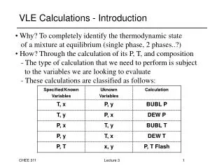
VLE Calculations - Introduction. Why? To completely identify the thermodynamic state of a mixture at equilibrium (single phase, 2 phases..?) How? Through the calculation of its P, T, and composition - The type of calculation that we need to perform is subject

VLE Calculations - Introduction
E N D
Presentation Transcript
VLE Calculations - Introduction • Why? To completely identify the thermodynamic state • of a mixture at equilibrium (single phase, 2 phases..?) • How? Through the calculation of its P, T, and composition • - The type of calculation that we need to perform is subject • to the variables we are looking to evaluate • - These calculations are classified as follows: Lecture 3
VLE Calculations – Introduction (cont’d) • As we are going to see later in the course, the aforementioned • VLE calculations are also applicable to non-ideal or/and • multi-component mixtures • For now, we are going to employ them only for the calculation • of the state and composition of binary and ideal mixtures • The calculations revolve around the use of 2 key equations: • 1) Raoult’s law for ideal phase behaviour: • 2) Antoine’s Equation (1) (2) Lecture 3
BUBL P Calculation (T, x1 known) • - Calculate and from Antoine’s Equation • For the vapour-phase composition (bubble) we can write: • y1+y2=1 (3) • Substitute y1 and y2 in Eqn (3) by using Raoult’s law: • (4) • - Re-arrange and solve Eqn. (4) for P • Now you can obtain y1 from Eqn (1) • Finally, y2 = 1-y1 Lecture 3
DEW P Calculation (T, y1 known) • - Calculate and from Antoine’s Equation • For the liquid-phase composition (dew) we can write: • x1+x2=1 (5) • Substitute x1 and x2 in Eqn (5) by using Raoult’s law: • (6) • - Re-arrange and solve Eqn. (6) for P • Now you can obtain x1 from Eqn (1) • Finally, x2 = 1-x1 Lecture 3
BUBL T Calculation (P, x1 known) • Since T is an unknown, the saturation pressures for the • mixture components cannot be calculated directly. Therefore, • calculation of T, y1 requires an iterative approach, as follows: • Re-arrange Antoine’s equation so that the saturation temperatures • of the components at pressure P can be calculated: • (7) • Select a temperature T’ so that • Calculate • Solve Eqn. (4) for pressure P’ • If , then P’=P; If not, try another T’-value • Calculate y1 from Raoult’s law Lecture 3
DEW T Calculation (P, y1 known) • Same as before, calculation of T, x1 requires an iterative approach: • Re-arrange Antoine’s equation so that the saturation temperatures • of the components at pressure P can be calculated from Eqn. (7): • - Select a temperature T’ so that • Calculate from Antoine’s Eqn. • Solve Eqn. (6) for pressure P’ • If , then P’=P; If not, try another T’-value • Calculate x1 from Raoult’s law Lecture 3
P, T Flash Calculation • - Calculate and from Antoine’s Equation • Use Raoult’s law in the following form: • (8) • - Re-arrange and solve Eqn. (8) for x1 • Now you can obtain y1 from Eqn (1), i.e., Lecture 3
Example • Assuming Roult’s Law to be valid, prepare • a Pxy diagram for T=90oC, and • a Txy diagram for P=90 kPa • for a mixture of 1-chlorobutane (1) /chlorobenzene (2) • Antoine Coefficients: Lecture 3
Construction of Pxy diagrams • The construction of Pxy diagram requires multiple P, T, Flash • calculations, each one of which provides a set of equilibrium y1, x1 • values for a given value of pressure (under constant T) • The results can be tabulated as shown below: Lecture 3
Example* – (a) Generation of Pxy Data *Slides1-4 (current lecture) correspond to the solution of the example problem presented in Lecture 3 (Slide 10) Lecture 3J.S. Parent
160.00 140.00 120.00 liquid 100.00 x1 P (kPa) 80.00 y1 VLE 60.00 40.00 vapor 20.00 0.00 0.00 0.20 0.40 0.60 0.80 1.00 Example – (a) Construction of a Pxy Plot Lecture 3J.S. Parent
Construction of Txy diagrams • The construction of Txy, diagram requires multiple P, T, Flash • calculations, each one of which provides a set of equilibrium y1, x1 • values for a given value of temperature (at fixed P) • The results can be tabulated as shown below: Lecture 3
Example – (b) Generation of Txy Data Lecture 3J.S. Parent
Example – (b) Construction of a Txy Plot Lecture 3J.S. Parent
What do we need to know so far? • How to use the Phase Rule (F=2-p+N) • How to read VLE charts • - Identify bubble point and dew point lines • - Read sat. pressures or temperatures from the chart • - Determine the state and composition of a mixture • How to perform Bubble Point, Dew Point, and P,T-Flash calculations • - Apply Raoult’s law • - Apply Antoine’s equation • How to use the Lever Rule (graphically or numerically) • How to construct VLE (Pxy or Txy ) charts for ideal mixtures Lecture 3