Download
1 / 28
280 likes | 317 Views
This presentation discusses the challenges and advancements in climate modeling at GFDL, focusing on natural climate variability, anthropogenic changes, and model developments to support NOAA's strategic goals. It reviews the projected global warming trends and contributions to IPCC reports, highlighting key issues and uncertainties in modeling. The text outlines the progress in understanding climate factors, modeling approaches, and future research questions to improve accuracy and predictions.

E N D
Climate Modeling at GFDL:The Scientific Challenges V. Ramaswamy NOAA/ Geophysical Fluid Dynamics Laboratory November 12, 2008
GFDL Mission Directly supports the DOC And NOAA Strategic Goals Be a world leader for the production of timely and reliable knowledge and assessments on natural climate variability and anthropogenic changes and in the development of the required earth system models. Work cooperatively in NOAA to advance its expert assessments of changes in national and global climate through research, improved models, and products. One of 2 Climate Modeling Centers called for in the US Climate Change Science Program [CCSP]
Atmospheric, Ocean, Land, Coupled, Earth System Model Developments Matrix Managed
GFDL’s Recent Major Climate Model Developments ESM 2.1 w/ OM3 {M,G} CM 2.4 B-grid FV core CM2.0 CM2.1 Hi-res AM2 CM3 FV, CS cores AM2, ----------- LM2, SIS, OM3 (MOM4) AM3, LM3, SIS, OM3 (MOM4, GOLD) CCSPs, NARCCAP AR4, WMO/UNEP 2001-2004 2005 2006 2007 2008
Anthro. RF > 0 (v. high conf.) Projected global warming NOAA/ GFDL model simulations contributed to IPCC AR4 AR4 conclusions 20th Cent. continental warming likely due to human activity Projected pattern of rainfall changes in 21st Cent. Projected warming pattern in early and late 21st Cent.
CCSP 3.3 Global decreases in sulfate aerosolwarmer U.S. summers in 2100 NOAA/ GFDL contribution to CCSP reports CCSP 1.1 dT (sfc - tropos): Models vs. Obs. CCSP 2.4 CCSP 3.2
OUTLINE • Understanding present climate; quantifying the causal factors and attribution of past climate change; and projections of future climate changes. • Challenges and progress in modeling the Atmosphere, Ocean, Coupled Atmosphere-Ocean, and Biosphere to address the key issues.
The World Has Warmed Globally averaged, the planet is about 0.75°C warmer than it was in 1860, based upon dozens of high-quality long records using thermometers worldwide, including land and ocean. Eleven of the last 12 years are among 12 warmest since 1850 in the global average. Globally averaged, the planet is ~0.75°C warmer than it was in 1860, based upon dozens of high-quality long records, including land and ocean. Eleven of the last 12 years are among 12 warmest since 1850 in the global average. IPCC AR4
GFDL Climate Model CM2.1 1950 2000 Nat = Natural Forcing Anth = Anthropogenic Forcing AllForc = (Nat + Anth) Forcings CRU = Observations IPCC AR4 simulation
Human and Natural Drivers of Climate Change IPCC (2007)
Anthropogenic forcings and response [1950-2000] GFDL CM 2.1
2000 1860
2000 1860
AOD GFDL CM2.1 (1996-2000) AOD overestimated (East coast) Sulfate AOD overestimated (Europe) Biomass emissions underestimated (S America) Biomass emissions underestimated (S Africa) Aerosol Optical Depths from GFDL Coupled Model 2.1 (CM2.1), AVHRR, and MODIS
The FutureWhat will be the impacts of changes in Greenhouse Gases and Aerosols?
Pollution controls How might future changes in aerosols affect climate? HISTORICAL and FUTURE SCENARIOS Emissions of Short-lived Gases and Aerosols (A1B) CO2 concentrations 60 50 40 30 20 10 NOx (Tg N yr-1) A1B IPCC, 2001 250 200 150 100 50 SO2 (Tg SO2 yr-1) ppmv 25 20 15 10 5 0 BC (Tg C yr-1) Large uncertainty in future emission trajectories for short-lived species Horowitz, JGR, 2006 1880 1920 1960 2000 2040 2080
Up to 40% of U.S. warming in summer (2090s-2000s) from short-lived species Results from GFDL Climate Model [Levy et al., 2008] From changing well-mixed greenhouse gases +short-lived species From changing only short-lived species Change in Summer Temperature 2090s-2000s (°C) Warming from increases in BC + decreases in sulfate; depends critically on highly uncertain future emission trajectories
New Science Questions for Next-Generation Model • What are the roles of aerosol-cloud interactions in climate and climate change? • How will land and ocean carbon cycles interact with climate change? • To what extent is decadal prediction possible? • What are the dominant chemistry-climate feedbacks?
Atmospheric Model Developments to Address the New Questions • Interactive chemistry to link emissions to aerosol composition • Aerosol activation requires super-saturation at cloud scale => Sub-grid PDFs of vertical velocity for convective and stratiform clouds • Sufficiently realistic tropical land precipitation for land carbon model • Stratospheric model for chemistry and links to troposphere, including those on multi-year scales relevant to decadal prediction
Water vapor band radiance error budget Overestimation Underestimation Window H2O vib-rot Model – satellite difference spectrum Total-sky MODEL-AIRS radiance difference [Huang et al. 2007 GRL]
Aerosol vs. Dynamics Aerosol Indirect Effects (1st and 2nd) Clean/Maritime Polluted/Continental Ramanathan et al. (2001)
T = 288 K p = 850 hPa Aerosol mass = { 0.5, 0.5, 0.5 } x 10-12 kg CCN activation is a non-linear function of vertical velocity from Ming et al. (2006, JAS)
Large Eddy Simulation shows small-scale activation. ~ 12.9 km updraft: activation downdraft: evaporation simulation by Chris Golaz
Layer-averaged activation: Because N* is non-linear However, Large-scale CCN activation
To use satellites to evaluate GCMs, the GCM must be sampled like the satellites OAR/CDC