Climate Modeling
Climate Modeling. Supercomputing Challenge Sandia National Laboratories March 19, 2007 Bill Spotz. My Background. University of Texas at Austin PhD, Aerospace Engineering Computational fluid dynamics High-order compact methods National Center for Atmospheric Research

Climate Modeling
E N D
Presentation Transcript
Climate Modeling Supercomputing Challenge Sandia National Laboratories March 19, 2007 Bill Spotz
My Background • University of Texas at Austin • PhD, Aerospace Engineering • Computational fluid dynamics • High-order compact methods • National Center for Atmospheric Research • Postdoc in Advanced Study Program • Project Scientist in Scientific Computing Division • High-order global atmospheric models • Sandia National Laboratories • Multiphysics coupling • Climate modeling
International Panel on Climate Change • United Nations org, ~2000 climate scientists • Issue report with ~7 year frequency • Latest report issued February, 2007 • Warming trend is undeniable • 90-99% certainty that humans contribute • IPCC climate modeling • Hundreds of simulations, several models • Models “frozen” in 2004 • 6-12 mo, debugging, tuning and understanding biases • ~1 yr, running simulations • ~1 yr, analyzing data…
US Climate Modeling • Community Climate System Model (CCSM) • National Science Foundation • Department of Energy • NASA • 500,000+ lines of FORTRAN
Example Climate Model Outputs Sources: http://www.vets.ucar.edu/vg/CCM3T170/index.shtml Earth Simulator Project
A Quick Diversion: Chaos Theory • Ed Lorenz, MIT meteorologist (1963) • VERY simple weather model • 3 variables • Found that small changes when “restarting” can drastically alter results • “Sensitivity to Initial Conditions” • Initial conditions for weather models come from measurements • Confidence in weather forecasts: ~5 days
Global Mean Temperature Anomaly Source: Meehl et al., J. Climate 17, 2004
Climate Modeling at Sandia • SciDAC (Scientific Discovery through Advanced Computing) • Focus on next generation of computers w/100,000s of processors • Atmospheric model is the bottleneck • New algorithms better suited to huge computers (petascale)
Computer Scaling Prefixes Uses: petabytes (memory) petaFLOPS (floating-point operations/sec)
Dynamics and Physics • Dynamics • Large scale motions in the atmosphere and ocean: winds, temperature and pressure • Accounts for almost all climate variability (large scale waves and turbulence) • Motion governed by the Euler equations, rotating frame, hydrostatic approximation, dissipation/turbulence model • Physics • Very small scale processes which force the dynamics mostly through heating and cooling • Radiation, clouds, vegetation, convection, precipitation • Accounts for most uncertainty in climate models
Resolution CCSM simulated years/day 400 23 300 8 150 4 IBM Power 5 System 200 CPUs
DOE Goal for Climate: 10km Resolution • Atmospheric Model • At 10km, the atmosphere will be the dominant component of a coupled model. • 10km is necessary to resolve regional detail of temperature and precipitation important for local and social impacts of climate change. • Many forecast models use 10km regional resolution and hydrostatic: could replace with a single global forecast model. • Ocean Model • 10km resolution required to be eddy-resolving (for those eddies that contain most of the kinetic energy in the ocean). • DOE SCaLeS Report • “An important long-term objective of climate modeling is to have the spatial resolution of the atmospheric and oceanic components both at ~1/10° (~ 10 km resolution at the Equator).”
Why 10km Resolution? Wintertime precipitation over the United States as simulated by CCM3 at three different horizontal resolutions (300, 75 and 50km), and in the VEMAP observational dataset. Both small- and large-scale (e.g. in southeastern U.S.) features of simulated precipitation appear to converge towards observations as the model resolution becomes finer. Source: Duffy, Govindasamy, Milovich, and Thompson, LLNL, http://eed.llnl.gov/cccm/hiresolu.html
Why 10km Resolution? 0.10° Source: Maltrud and McClean, Ocean Modelling 8, 2005 0.25° Observations
0.1º 0.1º and PBC Observations POP 1/10 Global Ocean Simulation on Sandia's RedStorm Maltrud (LANL), Taylor (SNL), Bryan (NCAR) McClean (LLNL) Peacock (U Chicago)
CCSM Ocean Model (POP)Running on Red Storm • In collaboration with Mat Maltrud (LANL), we performed two 10 year simulations on 5000 processors. • Simulation rate: 8 years/day • Resolution: 0.10º (3600x2400x40) 350M grid points. • Input/Output: 1.5TB • High resolution and partial bottom cells give improved results for Gulf Stream separation, NW corner, Agulhas rings and Kuroshio current
Regional Climate Modeling: Nested Grid Approach • Global model: ~ 150 km resolution • Regional model: typically 5-25 km resolution, boundary conditions come from global model • Example: hurricane forecasting ~ 10km
Atmospheric Model Dynamical Cores SEAM Finite Volumes Spherical Harmonics Parallel Scalability Suppression of “wiggles” Accuracy
Spherical Harmonics (Spectral Transform) • Uses lat-lon grid for transforms: • FFT (longitude) • Legendre (Latitude) • No Pole Problems • Isotropic representation of data • Bigger time steps • Excellent accuracy • Solutions have “wiggles” • Poor parallel scalability
Finite Volumes on a Latitude-Longitude Grid • Latitude-longitude grid • Pole problems: • Singular coordinate system • Non-isotropic representation of data • Small gridsmall time step • Low order of accuracy • “Wiggles” are suppressed • Good parallel scalability, ruined by techniques to handle pole problems
Finite Volumes on an Icosahedral Grid • No lat-lon grid • No pole problems • Nearly isotropic representation of data • Bigger time steps • Low-order accuracy • “Wiggles” are suppressed • Good parallel scalability
SEAM: Spectral Element Atmospheric Model • No lat-lon grid • No pole problems • Nearly isotropic representation of data • Bigger time step • Excellent accuracy • Solutions have “wiggles” • Excellent parallel scalability
SEAM on Red Storm • Simulation: breakdown of the polar stratospheric vortex. • Record setting resolution: 1B grid points, 13km horizontal resolution, running on 7200 processors of Red Storm • 1 TB of output. • Integration rate: 0.1 years/day • Projected integration rate on petascale supercomputer: 10 years/day.
Breakdown of the Polar Vortex • Model problem comes from research into the ozone layer • CFCs destroy ozone and a hole has appeared over south pole, but not the north • CFCs have been banned • Hole should disappear ~10-15 years • Highlights fact that wind patterns are different over north and south poles • At south pole, air gets trapped in a vortex • At north pole, these vortices break down • Cause is land/sea geometry