Database Query Processing: Optimization Techniques

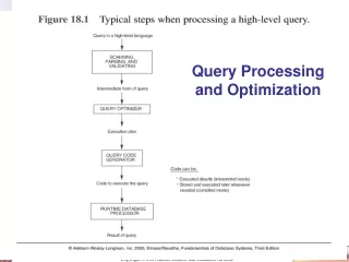
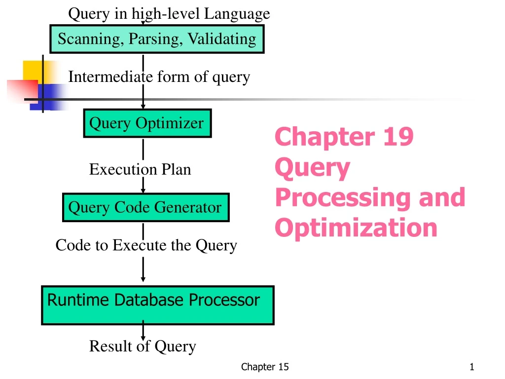
1. Runtime Database Processor Query in high-level Language Scanning, Parsing, Validating Chapter 19Query Processing and Optimization Intermediate form of query Query Optimizer Execution Plan Query Code Generator Code to Execute the Query Result of Query Chapter 15

2. <--SQL Query --> Syntactically Correct SQL Query --> Valid SQL Query --> Relational Algebra Query --> Optimized Relational Algebra Query --> Execution Plan --> Code for Query Query Optimization (Ricardo) Syntax Checking Validation Translation Relational Algebra Optimization Strategy Selection Code Generation Chapter 15

3. Oracle 11 g- The Query Optimizer http://docs.oracle.com/cd/B28359_01/server.111/b28274/optimops.htm#PFGRF001 Chapter 15

4. Techniques • Heuristic rules • reordering the operations in a query tree • Estimate the cost Chapter 15

5. Cost • Number and type of disk access required • Amount of internal and external memory needed • Process time requirement • Communication cost Chapter 15

6. 1. Translating SQL Queries into Relational Algebra (1) • Query block: • The basic unit that can be translated into the algebraic operators and optimized. • A query block contains a single SELECT-FROM-WHERE expression, as well as GROUP BY and HAVING clause if these are part of the block. • Nested queries within a query are identified as separate query blocks. • Aggregate operators in SQL must be included in the extended algebra. Chapter 15

7. Translating SQL Queries into Relational Algebra (2) SELECT LNAME, FNAME FROM EMPLOYEE WHERE SALARY > ( SELECT MAX (SALARY) FROM EMPLOYEE WHERE DNO = 5); SELECT LNAME, FNAME FROM EMPLOYEE WHERE SALARY > C SELECT MAX (SALARY) FROM EMPLOYEE WHERE DNO = 5 πLNAME, FNAME(σSALARY>C(EMPLOYEE)) ℱMAX SALARY(σDNO=5 (EMPLOYEE)) Chapter 15

8. SELECT Operations • OP1: ssn = 123456789(EMPLOYEE) • OP 2:  DNUMBER > 5(DEPARTMENT) • OP 3:  DNO = 5(EMPLOYEE) • OP 4:  DNO = 5 AND SALARY >3000 AND SEX = ‘F’ (EMPLOYEE) • OP 5: ESSN = 123456789 AND PNO = 10(WORKS_ON) Chapter 15

9. Chapter 15

10. Chapter 15

11. Chapter 15

12. Chapter 15

13. Implementing the SELECT Operations • S1 Linear search • S2 Binary tree • S3 Using a primary index or hash key to retrieve a single record • S4 Using a primary index to retrieve multiple records • S5 Using a clustering index to retrieve multiple records • S6 Using a secondary (B+ tree) index Chapter 15

14. Search Methods for Simple Selection •S1. Linear search (brute force):Retrieve every recordin the file, and test whether its attribute values satisfy the selection condition. •S2. Binary search:If the selection condition involves an equality comparison on a key attribute on which the file is ordered, binary search—which is more efficient than linear search—can be used. An example is OP1 if SSN is the ordering attribute for the EMPLOYEE file. •S3. Using a primary index (or hash key):If the selection condition involves an equality comparison on a key attribute with a primary index (or hash key)—for example, SSN = ‘123456789’ in OP1—use the primary index (or hash key) to retrieve the record. Note that this condition retrieves a single record (at most). Chapter 15

15. Search Methods for Simple Selection •S4. Using a primary index to retrieve multiple records:If the comparison condition is >, >=, <, or <= on a key field with a primary index—for example, DNUMBER > 5 in OP2—use the index to find the record satisfying the corresponding equality condition (DNUMBER = 5), then retrieve all subsequent records in the (ordered) file. For the condition DNUMBER < 5, retrieve all the preceding records. •S5. Using a clustering index to retrieve multiple records:If the selection condition involves an equality comparison on a non-key attribute with a clustering index—for example, DNO = 5 in OP3—use the index to retrieve all the records satisfying the condition. •S6. Using a secondary (-tree) index on an equality comparison:This search method can be used to retrieve a single record if the indexing field is a key (has unique values) or to retrieve multiple records if the indexing field is not a key.This can also be used for comparisons involving >, >=, <, or <=. Chapter 15

16. SELECT (Cont.) • S7. Conjunctive Selection • S8. Conjunctive selection using a composite index (two or more attributes) • S9. Conjunctive selection by intersection of record pointers (secondary indexes need more than two attributes) Chapter 15

17. Search Methods for Complex Selection If a condition of a SELECT operation is a conjunctive condition—that is, if it is made up of several simple conditions connected with the AND logical connective such as OP4 above—the DBMS can use the following additional methods to implement the operation: • S7. Conjunctive selection using an individual index: If an attribute involved in any single simple condition in the conjunctive condition has an access path that permits the use of one of the Methods S2 to S6, use that condition to retrieve the records and then check whether each retrieved record satisfies the remaining simple conditions in the conjunctive condition. • S8. Conjunctive selection using a composite index: If two or more attributes are involved in equality conditions in the conjunctive condition and a composite index (or hash structure) exists on the combined fields—for example, if an index has been created on the composite key (ESSN, PNO) of the WORKS_ON file for OP5—we can use the index directly. • S9. Conjunctive selection by intersection of record pointers (Note 8): If secondary indexes (or other access paths) are available on more than one of the fields involved in simple conditions in the conjunctive condition, and if the indexes include record pointers (rather than block pointers), then each index can be used to retrieve the set of record pointers that satisfy the individual condition. The intersection of these sets of record pointers gives the record pointers that satisfy the conjunctive condition, which are then used to retrieve those records directly. If only some of the conditions have secondary indexes, each retrieved record is further tested to determine whether it satisfies the remaining conditions (Note 9). Chapter 15

18. Join Operations • J1. Nested (inner-outer) loop • J2. Single-loop join--Using an access structure to retrieve the matching records (hashing) • J3. Sort-merge join (Tables are physically sorted) • J4. Hash-join Chapter 15

19. Methods for Implementing Joins (R |X|A=BS) • J1. Nested-loop join (brute force):For each record t in R (outer loop), retrieve every record s from S (inner loop) and test whether the two records satisfy the join condition t[A] = s[B]. • J2. Single-loop join (using an access structure to retrieve the matching records): If an index (or hash key) exists for one of the two join attributes—say, B of S—retrieve each record t in R, one at a time (single loop), and then use the access structure to retrieve directly all matching records s from S that satisfy s[B] = t[A]. Chapter 15

20. Methods for Implementing Joins (R |X|A=BS) ..cont. • J3 Sort–merge join: If the records of R and S are physically sorted (ordered) by value of the join attributes A and B, respectively, --Both files are scanned concurrently in order of the join attributes, matching the records that have the same values for A and B. If the files are not sorted, they may be sorted first by using external sorting. Chapter 15

21. Methods for Implementing Joins (R |X|A=BS) ..cont. • J4. Hash-join: • The records of files R and S are both hashed to the same hash file, using the same hashing function on the join attributes A of R and B of S as hash keys. First, a single pass through the file with fewer records (say, R) hashes its records to the hash file buckets; this is called the partitioning phase, since the records of R are partitioned into the hash buckets. In the second phase, called the probingphase, a single pass through the other file (S) then hashes each of its records to probe the appropriate bucket, and that record is combined with all matching records from R in that bucket. This simplified description of hash-join assumes that the smaller of the two files fits entirely into memory buckets after the first phase. We will discuss variations of hash-join that do not require this assumption below. Chapter 15

22. Project Operations • Keep the required attributes (columns) • If <attribute list> does not include a key of R, duplicate tuples must be eliminated Chapter 15

23. Using Heuristics • Apply SELECT AND PROJECT operations before applying the JOIN and other binary operations Chapter 15

24. Transformation Rules(p. 611) 1. Cascade of  2. Commutativity of  3. Cascade of  4. Commuting of  with  5. Commutativity of |X| 6. Commuting of  and |X| 7. Commuting of  with |X| 8. Commutativity of set operation 9. Associativity of |X|, X, , and  Chapter 15

25. Transformation Rules (cont.) 10. Commuting  with set operations 11. The operation commutes with  12. Other transformations (DeMorgan’s laws) Chapter 15

26. EXAMPLE (Q2) SELECT P.PNUMBER, P.DNUM, E.LNAME, E.ADDRESS, E.BDATE FROM PROJECT P, DEPARTMENT D, EMPLOYEE E WHERE P.DNUM = D AND D.MSGR = E.SSN AND P.PLOCATION = ‘Stafford’; Chapter 15

27. SELECT P.PNUMBER, P.DNUM, E.LNAME, E.ADDRESS, E.BDATE FROM PROJECT P, DEPARTMENT D, EMPLOYEE E WHERE P.DNUM = D AND D.MSGR = E.SSN AND P.PLOCATION = ‘Stafford’; Chapter 15

28. Using Heuristics in Query Optimization (6) • Heuristic Optimization of Query Trees: • The same query could correspond to many different relational algebra expressions — and hence many different query trees. • The task of heuristic optimization of query trees is to find a final query tree that is efficient to execute. • Example: Q: SELECT LNAME FROM EMPLOYEE, WORKS_ON, PROJECT WHERE PNAME = ‘AQUARIUS’ AND PNMUBER=PNO AND ESSN=SSN AND BDATE > ‘1957-12-31’; Chapter 15

29. Using Heuristics in QueryOptimization (7) SELECT LNAME FROM EMPLOYEE, WORKS_ON, PROJECT WHERE PNAME = ‘AQUARIUS’ AND PNUMBER=PNO AND ESSN=SSN AND BDATE > ‘1957-12-31’; Chapter 15

30. Using Heuristics in Query Optimization (8) Chapter 15

31. Chapter 15

32. Retrieve the names of all employees in department 5 who work more than 10 hours per week on the 'ProductX' project. Chapter 15

33. 18.4.1 Cost Components for Query Execution • The cost of executing a query • Access cost to secondary storage: --cost of searching for, reading, and writing data blocks that reside on secondary storage, mainly on disk. • Storage cost: -- cost of storing any intermediate files that are generated by an execution strategy for the query. • Computation cost:-- cost of performing in-memory operations on the data buffers during query execution. -- searching for and sorting records, merging records for a join, and performing computations on field values. • Memory usage cost:This is the cost pertaining to the number of memory buffers needed during query execution. • Communication cost: --cost of shipping the query and its results from the database site to the site or terminal where the query originated. Chapter 15

34. Information needed • In DBMS catalog • number of records (tuples) (r) • the (average) record size (R), • number of blocks (b) (or close estimates of them) are needed • blocking factor (bfr) • number of levels (x) of each multilevel index (primary, secondary, or clustering) Chapter 15

35. Links • http://en.wikipedia.org/wiki/Query_optimizer • http://en.wikipedia.org/wiki/Query_plan • http://redbook.cs.berkeley.edu/redbook3/lec7.html Chapter 15