Introduction to Query Processing and Query Optimization Techniques
Introduction to Query Processing and Query Optimization Techniques. Introduction to Query Processing. Query optimization : The process of choosing a suitable execution strategy for processing a query. Amongst all equivalent evaluation plans choose the one with lowest cost.


Introduction to Query Processing and Query Optimization Techniques
E N D
Presentation Transcript
Introduction to Query Processing and Query Optimization Techniques
Introduction to Query Processing • Query optimization: • The process of choosing a suitable execution strategy for processing a query. • Amongst all equivalent evaluation plans choose the one with lowest cost. • Cost is estimated using statistical information from the database catalog • e.g. number of tuples in each relation, size of tuples • Two internal representations of a query: • Query Tree • Query Graph
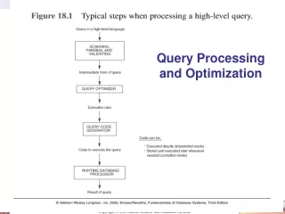
Basic Steps in Query Processing • Select balance From account where balance < 2500 • balance2500(balance(account)) is equivalent to • balance(balance2500(account)) • Annotated relational algebra expression specifying detailed evaluation strategy is called an evaluation-plan. • E.g., can use an index on balance to find accounts with balance 2500, • or can perform complete relation scan and discard accounts with balance 2500
Measures of Query Cost • Cost is generally measured as total elapsed time for answering query. Many factors contribute to time cost • disk accesses, CPU, or even network communication • Typically disk access is the predominant cost, and is also relatively easy to estimate. • For simplicity we just use number of block transfers from disk as the cost measure • Costs depends on the size of the buffer in main memory • Having more memory reduces need for disk access
Translating SQL Queries into Relational Algebra • Query Block: • The basic unit that can be translated into the algebraic operators and optimized. • A query block contains a single SELECT-FROM-WHERE expression, as well as GROUP BY and HAVING clause if these are part of the block. • Nested queries within a query are identified as separate query blocks • Aggregate operators in SQL must be included in the extended algebra.
Translating SQL Queries into Relational Algebra SELECT LNAME, FNAME FROM EMPLOYEE WHERE SALARY > ( SELECT MAX (SALARY) FROM EMPLOYEE WHERE DNO = 5); SELECT LNAME, FNAME FROM EMPLOYEE WHERE SALARY > C SELECT MAX (SALARY) FROM EMPLOYEE WHERE DNO = 5 πLNAME, FNAME(σSALARY>C(EMPLOYEE)) ℱMAX SALARY(σDNO=5 (EMPLOYEE))
Algorithms for External Sorting • Sorting is needed in • Order by, join, union, intersection, distinct, … • For relations that fit in memory, techniques like quicksort can be used. • External sorting: • Refers to sorting algorithms that are suitable for large files of records stored on disk that do not fit entirely in main memory, such as most database files. • For relations that don’t fit in memory, external sort-merge is a good choice
External Sort-Merge • External sort-merge algorithm has two steps: • Partial sort step, called runs. • Merge step, merges the sorted runs. • Sort-Merge strategy: • Starts by sorting small subfiles (runs) of the main file and then merges the sorted runs, creating larger sorted subfiles that are merged in turn. • Sorting phase: • Sorts nB pages at a time • nB = # of main memory pages buffer • creates nR = b/nBinitialsorted runs on disk • b = # of file blocks (pages) to be sorted • Sorting Cost = read b blocks + write b blocks = 2 b
External Sort-Merge • Example: • nB = 5 blocks and file size b = 1024 blocks, then • nR = (b/nB) = 1024/5 = 205 initial sorted runs each of size 5 bocks (except the last run which will have 4 blocks) nB = 2, b = 7, nR = b/nB = 4 run
External Sort-Merge • Sort Phase: creates nR sorted runs. i = 0 Repeat Read next nB blocks into RAM Sort the in-memory blocks Write sorted data to run file Ri i = i + 1 Until the end of the relation nR = i
External Sort-Merge • Merging phase: • The sorted runs are merged during one or more passes. • The degree of merging (dM) is the number of runs that can be merged in each pass. • dM = Min (nB-1, nR) • nP = (logdM(nR)) • nP: number of passes. • In each pass, • One buffer block is needed to hold one block from each of the runs being merged, and • One block is needed for containing one block of the merged result.
External Sort-Merge • We assume (for now) that nRnB. • Merge the runs (nR-way merge). • Use nR blocks of memory to buffer input runs, and 1 block to buffer output. • Merge nR Runs Step Read 1st block of each nR runs Ri into its buffer page Repeat Select 1st record (sort order) among nR buffer pages Write the record to the output buffer. If the output buffer is full write it to disk Delete the record from its input buffer page If the buffer page becomes empty then read the next block (if any) of the run into the buffer Until all input buffer pages are empty
External Sort-Merge • Merge nB- 1 Runs Step • If nR nB, several merge passes are required. • merge a group of contiguous nB- 1 runs using one buffer for output • A pass reduces the number of runs by a factor of nB- 1, and creates runs longer by the same factor. • E.g. If nB = 11, and there are 90 runs, one pass reduces the number of runs to 9, each 10 times the size of the initial runs • Repeated passes are performed till all runs have been merged into one
External Sort-Merge • Degree of merging (dM) • # of runs that can be merged together in each pass = min (nB - 1, nR) • Number of passes nP = (logdM(nR)) • In our example • dM = 4 (four-way merging) • min (nB-1, nR) = min(5-1, 205) = 4 • Number of passes nP = (logdM(nR)) = (log4(205)) = 4 • First pass: • 205 initial sorted runs would be merged into 52 sorted runs • Second pass: • 52 sorted runs would be merged into 13 • Third pass: • 13 sorted runs would be merged into 4 • Fourth pass: • 4 sorted runs would be merged into 1
External Sort-Merge Blocking factor bfr = 1 record, nB = 3, b = 12, nR = 4, dM = min(3-1, 4) = 2
External Sort-Merge • External Sort-Merge: Cost Analysis • Disk accesses for initial run creation (sort phase) as well as in eachmergepass is 2b • reads every block once and writes it out once • Initial # of runs is nR = b/nB and # of runs decreases by a factor of nB - 1 in each merge pass, then the total # of merge passes is np = logdM(nR) • In general, the cost performance of Merge-Sort is • Cost = sort cost + merge cost • Cost = 2b + 2b * np • Cost = 2b + 2b * logdM nR • =2b(logdM(nR) + 1)
Catalog Information • File • r: # of records in the file • R: record size • b: # of blocks in the file • bfr: blocking factor • Index • x: # of levels of a multilevel index • bI1: # of first-level index blocks
Catalog Information • Attribute • d: # of distinct values of an attribute • sl (selectivity): • the ratio of the # of records satisfying the condition to the total # of records in the file. • s (selection cardinality) = sl * r • average # of records that will satisfy an equality condition on the attribute • For a key attribute: • d = r, sl = 1/r, s = 1 • For a nonkey attribute: • assuming that d distinct values are uniformly distributed among the records • the estimated sl = 1/d, s = r/d
File Scans • Types of scans • File scan – search algorithms that locate and retrieve records that fulfill a selection condition. • Index scan – search algorithms that use an index • selection condition must be on search-key of index. • Cost estimate C = # of disk blocks scanned
Algorithms for SELECT Operations • Implementing the SELECT Operation • Examples: • (OP1): SSN='123456789' (EMP) • (OP2): DNUMBER>5(DEPT) • (OP3): DNO=5(EMP) • (OP4): DNO=5 AND SALARY>30000 AND SEX=F(EMP) • (OP5): ESSN=123456789 AND PNO=10(WORKS_ON)
Algorithms for Selection Operation • Search Methods for Simple Selection: • S1 (linear search) • Retrieve every record in the file, and test whether its attribute values satisfy the selection condition. • If selection is on a nonkey attribute, C = b • If selection is equality on a key attribute, • if record found, average cost C = b/2, else C = b
Algorithms for Selection Operation • S2 (binary search) • Applicable if selection is an equality comparison on the attribute on which file is ordered. • Assume that the blocks of a relation are stored contiguously • If selection is on a nonkey attribute: • C = log2b: cost of locating the 1st tuple + • s/bfr - 1: # of blocks containing records that satisfy selection condition • If selection is equality on a key attribute: • C = log2b, since s = 1, in this case
Selections Using Indices • S3 (primary or hash index on a key, equality) • Retrieve a single record that satisfies the corresponding equality condition • If the selection condition involves an equality comparison on a key attribute with a primary index (or a hash key), use the primary index (or the hash key) to retrieve the record. • Primary index: retrieve 1 more block than the # of index levels, • C = x + 1: • Hash index: • C =1: for static or linear hashing • C =2: for extendable hashing
Selections Using Indices • S4 (primary index on a key, range selection) • S4 Using a primary index to retrieve multiple records: • If the comparison condition is >, ≥, <, or ≤ on a key field with a primary index, use the index to find the record satisfying the corresponding equality condition, then retrieve all subsequent records in the (ordered) file. • Assuming relation is sorted on A • For Av(r) use index to find 1st tuple = v and retrieve all subsequent records. • For Av(r) use index to find 1st tuple = v and retrieve all preceding records. • OR just scan relation sequentially till 1st tuple v;do not use index with average cost C = b/2 • Average costC = x + b/2
Selections Using Indices • S5 (clustered index on nonkey, equality) • Retrieve multiple records. • Records will be on consecutive blocks • C = x + s/bfr • # of blocks containing records that satisfy selection condition
Selections Using Indices • S6-1 (secondary index B+-tree, equality) • Retrieve a single record if the search-key is a candidate key, • C = x + 1 • Retrieve multiple records if search-key is not a candidate key, • C = x + s • Can be very expensive!. Each record may be on a different block , one block access for each retrieved record
Selections Using Indices • S6-2 (secondary index B+-tree, comparison) • For Av(r) use index to find 1st index entry = v and scan index sequentially from there, to find pointers to records. • For Av(r) just scan leaf pages of index finding pointers to records, till first entry v • If ½ records are assumed to satisfy the condition, then ½ first-level index blocks are accessed, plus ½ the file records via the index • C = x + bI1/2 + r/2
Complex Selections: 12…n(r) • S7 (conjunctive selection using one index) • Select i and algorithms S1 through S6 that results in the least cost for i(r). • Test other conditions on tuple after fetching it into memory buffer. • Cost of the algorithms chosen.
Complex Selections: 12…n(r) • S8 (conjunctive selection using composite index). • If two or more attributes are involved in equality conditions in the conjunctive condition and a composite index (or hash structure) exists on the combined field, we can use the index directly. • Use appropriate composite index if available using one the algorithms S3 (primary index), S5, or S6 (B+-tree, equality).
Complex Selections: 12…n(r) • S9 (conjunctive selection by intersection of record pointers) • Requires indices with record pointers. • Use corresponding index for each condition, and take intersection of all the obtained sets of record pointers, then fetch records from file • If some conditions do not have appropriate indices, apply test in memory. • Cost is the sum of the costs of the individual index scan plus the cost of retrieving records from disk.
Complex Selections: 12… n(r) • S10 (disjunctive selection by union of identifiers) • Applicable if all conditions have available indices. • Otherwise use linear scan. • Use corresponding index for each condition, and take union of all the obtained sets of record pointers. Then fetch records from file • READ • “Examples of Using the Cost Functionst” • page 569--570. • page 694-695
DuplicateElimination • Duplicate elimination can be implemented via hashing or sorting. • On sorting, duplicates will come adjacent to each other, and all but one set of duplicates can be deleted. • Optimization: duplicates can be deleted during run generation as well as at intermediate merge steps in external sort-merge. • Cost is the same as the cost of sorting • Hashing is similar – duplicates will come into the same bucket.
Algorithms for PROJECT Operation • Algorithm for PROJECT operations (Figure 15.3b) <attribute list>(R) • If <attribute list> has a key of relation R, extract all tuples from R with only the values for the attributes in <attribute list>. • If <attribute list> does NOT include a key of relation R, duplicated tuples must be removed from the results.
Algorithms for SET Operations • Algorithm for SET operations • Set operations: • UNION, INTERSECTION, SET DIFFERENCE and CARTESIAN PRODUCT • CARTESIAN PRODUCT of relations R and S include all possible combinations of records from R and S. The attribute of the result include all attributes of R and S. • Cost analysis of CARTESIAN PRODUCT • If R has n records and j attributes and S has m records and k attributes, the result relation will have n*m records and j+k attributes. • CARTESIAN PRODUCT operation is veryexpensive and should be avoided if possible.
Set Operations • R S: (See Figure 18.3c) • 1. Sort the two relations on the same attributes. • 2. Scan and merge both sorted files concurrently, whenever the same tuple exists in both relations, only one is kept in the merged results. • R S: (See Figure 18.3d) • 1. Sort the two relations on the same attributes. • 2. Scan and merge both sorted files concurrently, keep in the merged results only those tuples that appear in both relations. • R – S: (See Figure 18.3e) • keep in the merged results only those tuples that appear in relation R but not in relation S.
Aggregate Operations • The aggregate operations MIN, MAX, COUNT, AVERAGE, and SUM can be computed by scanning the whole records (the worst case) • If index exists on the attribute of MAX , MIN operation, then these operations can be done in a much more efficient way: select max/min (salary) from employee • If an (ascending) index on SALARY exists for the employee relation, then the optimizer could decide on traversing the index for the largest/smallest value, which would entail following the right/left most pointer in each index node from the root to a leaf.
Aggregate Operations • SUM, COUNT and AVG • For a dense index (each record has one index entry): • Apply the associated computation to the values in the index. • For a non-dense index: • Actual number of records associated with each index entry must be accounted for • With GROUP BY: the aggregate operator must be applied separately to each group of tuples. • Use sorting or hashing on the group attributes to partition the file into the appropriate groups; • Computes the aggregate function for the tuples in each group. • What if we have Clustering index on the grouping attributes?
Combining Operations using Pipelining • Motivation • A query is mapped into a sequence of operations. • Each execution of an operation produces a temporary result (Materialization). • Generating & saving temporary files on disk is time consuming. • Alternative: • Avoid constructing temporary results as much as possible. • Pipeline the data through multiple operations • pass the result of a previous operator to the next without waiting to complete the previous operation.
Materialization • Materialized evaluation: • evaluate one operation at a time, starting at the lowest-level. • Use intermediate results materialized into temporary relations to evaluate next-level operations.
Pipelining • Pipelined evaluation • evaluate several operations simultaneously, passing the results of one operation on to the next. • E.g., in previous expression tree, don’t store result of • instead, pass tuples directly to the join. • Similarly, don’t store result of join, pass tuples directly to projection. • Much cheaper than materialization: • no need to store a temporary relation to disk. • Pipelining may not always be possible • e.g., sort, hash-join.
Using Heuristics in Query Optimization • Process for heuristics optimization • The parser of a high-level query generates an initial internal representation; • Apply heuristics rules to optimize the internal representation. • A query execution plan is generated to execute groups of operations based on the access paths available on the files involved in the query. • The main heuristic is to apply first the operations that reduce the size of intermediate results. • E.g., Apply SELECT and PROJECT operations before applying the JOIN or other binary operations.
Using Heuristics in Query Optimization • Query tree: • A tree data structure that corresponds to a relational algebra expression. It represents the input relations of the query as leaf nodes of the tree, and represents the relational algebra operations as internal nodes. • An execution of the query tree consists of executing an internal node operation whenever its operands are available and then replacing that internal node by the relation that results from executing the operation. • Query graph: • A graph data structure that corresponds to a relational calculus expression. It does not indicate an order on which operations to perform first. There is only a single graph corresponding to each query.
Using Heuristics in Query Optimization • Example: • For every project located in ‘Stafford’, retrieve the project number, the controlling department number and the department manager’s last name, address and birthdate. • Relation algebra: PNUMBER, DNUM, LNAME, ADDRESS, BDATE (((PLOCATION=‘STAFFORD’(PROJECT))DNUM=DNUMBER (DEPARTMENT)) MGRSSN=SSN (EMPLOYEE)) • SQL query: Q2: SELECT P.NUMBER,P.DNUM,E.LNAME, E.ADDRESS, E.BDATE FROM PROJECT AS P,DEPARTMENT AS D, EMPLOYEE AS E WHERE P.DNUM=D.DNUMBER AND D.MGRSSN=E.SSN AND P.PLOCATION=‘STAFFORD’;