Query Processing and Optimization
Query Processing and Optimization. Introduction. Users are expected to write “efficient” queries. But they do not always do that! Users typically do not have enough information about the database to write efficient queries. E.g., no information on table size

Query Processing and Optimization
E N D
Presentation Transcript
Introduction • Users are expected to write “efficient” queries. But they do not always do that! • Users typically do not have enough information about the database to write efficient queries. E.g., no information on table size • Users would not know if a query is efficient or not without knowing how the DBMS’s query processor work • DBMS’s job is to optimize the user’s query by: • Converting the query to an internal representation (tree or graph) • Evaluate the costs of several possible ways of executing the query and find the best one.
Join Employee Project Join Employee and Project using hash join, … ... Steps in Query Processing SQL query Query Parsing Parse Tree Query Optimization Execution Plan Code Generation Runtime DB Processor Result Code
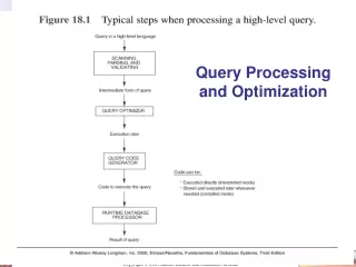
Query Processing Query in a high level language Scanning, Parsing, & Validating Intermediate form of query QUERY OPTIMIZER Execution Plan Query Code Generator Code to execute the query Runtime DB Processor Result of query
Basic Steps in Query Processing 1. Parsing and translation 2. Optimization 3. Evaluation
Basic Steps in Query Processing • Parsing and translation • translate the query into its internal form. (relational algebra) • Parser checks syntax, verifies relations • Evaluation • The query-execution engine takes a query-evaluation plan, executes that plan, and returns the answers to the query.
Query Processing • Consider the query: select balance from account where balance<2500 • Can be translated into either of the following RA expressions: balance2500(balance(account))balance(balance2500(account)) • The RA expressions are equivalent
Query Processing • Each relational algebra operation can be evaluated using one of several different algorithms • Correspondingly, a relational-algebra expression can be evaluated in many ways. • Annotated expression specifying detailed evaluation strategy is called an evaluation-plan • E.g., can use an index on balance to find accounts with balance < 2500, • or can perform complete relation scan and discard accounts with balance 2500
Query Optimization • Amongst all equivalent evaluation plans choose the one with lowest cost. • Cost is estimated using statistical information from the database catalog • e.g. number of tuples in each relation, size of tuples, etc. • First we need to learn: • How to measure query costs • Algorithms for evaluating relational algebra operations • How to combine algorithms for individual operations in order to evaluate a complete expression • How to optimize queries, that is, how to find an evaluation plan with lowest estimated cost
Measures of Query Cost • Cost is generally measured as total elapsed time for answering query • Many factors contribute to time cost • disk accesses, CPU, or even network communication • Typically disk access is the predominant cost, and is also relatively easy to estimate. Measured by taking into account • Number of seeks * average-seek-cost + Number of blocks read * average-block-read-cost + Number of blocks written * average-block-write-cost • Cost to write a block is greater than cost to read a block • data is read back after being written to ensure that the write was successful • Assumption: single disk • Can modify formulae for multiple disks/RAID arrays • Or just use single-disk formulae, but interpret them as measuring resource consumption instead of time
Measures of Query Cost (Cont.) • For simplicity we just use the number of block transfers from disk and the number of seeks as the cost measures • tT – time to transfer one block • tS – time for one seek • Cost for b block transfers plus S seeksb * tT + S * tS • We ignore CPU costs for simplicity • Real systems do take CPU cost into account • We do not include cost to writing output to disk in our cost formulae • Several algorithms can reduce disk I/O by using extra buffer space • Amount of real memory available to buffer depends on other concurrent queries and OS processes, known only during execution • We often use worst case estimates, assuming only the minimum amount of memory needed for the operation is available • Required data may be buffer resident already, avoiding disk I/O • But hard to take into account for cost estimation
Statistics and Catalogs • For each Table • Table name, file name (or some identifier) & file structure (e.g., heap file) • Attribute name and type of each attribute • Index name of each index • Integrity constraints • For each Index • Index name & the structure (e.g., B+ tree) • Search key attributes • For each View • View name & definition
Statistics and Catalogs • Cardinality: NTuples(N) for each R • Size: NPages(R) for each R • Index Cardinality: Number of distinct key values NKeys(I) for each I • Index Size: INPages(I) for each index I • For B+ tree index, INPages is number of leaf pages • Index Height: Number of non-leaf levels IHeight(I) for eact tree index • Index Range: ILow(I) & IHigh(I)
Statistics and Catalogs • Catalogs updated periodically • Updating whenever data changes is too expensive • More detailed information (e.g., histograms of the values in some field) are sometimes stored.
Operator Evaluation Algorithms for evaluating relational operators use some simple ideas extensively: • Indexing: If a selection or join condition is specified, use an index to examine just the tuples that satisfy the condition. • Iteration: Sometimes, faster to scan all tuples even if there is an index. (And sometimes, we can scan the data entries in an index instead of the table itself.) • Partitioning: By using sorting or hashing, we can partition the input tuples and replace an expensive operation by similar operations on smaller inputs.
Access Paths • An access path is a method of retrieving tuples: • File scan, or index that matches a selection (in the query) • A tree index matches (a conjunction of) terms that involve only attributes in a prefix of the search key. • E.g., Tree index on <a, b, c> matches the selection a=5 AND b=3, and a=5 AND b>6, but not b=3. • A hash index matches (a conjunction of) terms that has a term attribute = value for every attribute in the search key of the index. • E.g., Hash index on <a, b, c> matches a=5 AND b=3 AND c=5; but it does not match b=3, or a=5 AND b=3, or a>5 AND b=3 AND c=5.
Access Paths • Selectivity: Number of pages retrieved (Index + data) to retrieve all desired tuples • Using the most selective access path minimizes the cost of data retrieval • Reduction Factor: • Each conjunct is a filter • Fraction of tuples satisfying a given conjunct is called the reduction factor
Query Optimization • Techniques used by a DBMS to process, optimize, and execute high-level queries • A high-level query is • Scanned • Parsed • Validated • Internal representation • QUERY TREE • QUERY GRAPH • Many Execution Strategies • Choosing a suitable one for processing a query is QUERY OPTIMIZATION • Ideally: Want to find best plan • Practically: Avoid worst plans!
Query Optimization • Scanning • The scanner identifies the language tokens, such as SQL keywords, attribute names, & relation names • Parsing • Parser checks the query syntax to determine whether it is formulated according to the grammar rules of the query language • Validating • Checking that all the attribute & relation names are valid and semantically meaningful names in the schema of the particular DB being queried
SQL Queries to Relational Algebra • SQL queries are optimized by decomposing them into a collection of smaller units, called blocks • Query optimizer concentrates on optimizing a single block at a time
Translating SQL Queries into Relational Algebra • Query block: the basic unit that can be translated into the algebraic operators and optimized. • A query block contains a single SELECT-FROM-WHERE expression, as well as GROUP BY and HAVING clause if these are part of the block. • Nested queries within a query are identified as separate query blocks. • Aggregate operators in SQL must be included in the extended algebra.
Translating SQL Queries into Relational Algebra SELECT LNAME, FNAME FROM EMPLOYEE WHERE SALARY > ( SELECT MAX (SALARY) FROM EMPLOYEE WHERE DNO = 5); SELECT LNAME, FNAME FROM EMPLOYEE WHERE SALARY > C SELECT MAX (SALARY) FROM EMPLOYEE WHERE DNO = 5 πLNAME, FNAME(σSALARY>C(EMPLOYEE)) ℱMAX SALARY(σDNO=5 (EMPLOYEE))
Select Operation • File scan scan all records of the file to find records that satisfy selection condition • Binary search when the file is sorted on attributes specified in the selection condition • Index scan usingindex to locate the qualified records • Primary index, single record retrieval equality comparison on a primary key attribute with a primary index • Primary index, multiple records retrieval comparison condition <, >, etc. on a key field with primary index • Clustering index to retrieve multiple records • Secondary index to retrieve single or multiple records
Composite index EmpNo Age Complete Employee Records 012 25 123 30 Conjunctive Conditions • OP1 AND OP2 (e.g., EmpNo=123 AND Age=30) • Conjunctive selection: Evaluate the condition that has an index created (i.e., that can be evaluated very fast), get the qualified tuples and then check if these tuples satisfy the remaining conditions. • Conjunctive selection using composite index: if there is a composite index created on attributes involved in one or more conditions, then use the composite index to find the qualified tuples • Conjunctive selection by intersection of record pointers: if secondary indexes are available, evaluate each condition and intersect the sets of record pointers obtained.
Conjunctive Conditions • When there are more than one attribute with an index: • use the one that costs least, and • the one that returns the smallest number of qualified tuple • selectivity of a condition is the number of tuples that satisfy the condition divided by total number of tuples. • The smaller the selectivity, the fewer the number of tuples retrieved, and the higher the desirability of using that condition to retrieve the records. • Disjunctive select conditions: OP1 or OP2 are much more costly: • potentially a large number of tuples will qualify • costly if any one of the condition doesn’t have an index created
Join Operation • Join is one of the most time-consuming operations in query processing. • Two-way join is a join of two relations, and there are many algorithms to evaluate the join. • Multi-way join is a join of more than two relations; different orders of evaluating a multi-way join have different speeds • We shall study methods for implementing two-way joins of form R A=B S
m tuples in R R S 0005 n tuples in S 0005 0002 0002 0004 0002 0002 0003 0002 m*n checkings 0002 0001 0005 0005 Join Algorithm: Nested (inner-outer) Loop R A=B S • Nested (inner-outer) Loop: For each record r in R (outer loop), retrieve every record s from S (inner loop) and check if r[A] = s[B]. for each tuple r in R do for each tuple s in S do if r.[A] = s[B] then output result end end R and S can be reversed
R 0005 index on S S 0005 0002 0002 0004 0002 0002 0003 0002 0002 0001 0005 0005 When One Join Attributes is Indexed • If an index (or hash key) exists, say, on attribute B of S, should we put R in the outer loop or S? Why? • Records in the outer relation are accessed sequentially, an index on the outer relation doesn’t help; • Records in the inner relations are accessed randomly, so an index can retrieve all records in the inner relation that satisfy the join condition.
0001 0002 0002 0002 0002 0002 0002 0004 0003 0005 0005 0005 0005 Sort-Merge Join R A=B S • Sort-merge join: if the records of R and S are sorted on the join attributes A and B, respectively, then the relations are scanned in say ascending order, matching the records that have same values for A and B. • R and S are only scanned once. • Even if the relations are not sorted, it is better to sort them first and do sort-merge join then doing double-loop join. • if R and S are sorted, n + m • if not sorted:n log(n) + m log(m) + m + n
0001 0003 0005 0001 0002 0002 0002 0005 0002 0002 0002 0002 0002 0002 0002 0002 0002 0003 0004 0004 0005 0005 0005 0005 0005 0005 Hash Join Method • Hash-join: R and S are both hashed to the same hash file based on the join attributes. Tuples in the same bucket are then “joined”.
Hints on Evaluating Joins • Disk accesses are based on blocks, not individual tuples • Main memory buffer can significantly reduce the number of disk accesses • Use the smaller relation in outer loop in nested loop method • Consider if 1 buffer is available, 2 buffers, m buffers • When index is available, either the smaller relation or the one with large number of matching tuples should be used in the outer loop. • If join attributes are not indexed, it may be faster to create the indexes on-the-fly (hash-join is close to generating a hash index on-the-fly) • Sort-Merge is the most efficient; the relations are often sorted already • Hash join is efficient if the hash file can be kept in the main memory