Query processing and optimization

1. Query processing and optimization These slides are a modified version of the slides of the book “Database System Concepts” (Chapter 13 and 14), 5th Ed., McGraw-Hill, by Silberschatz, Korth and Sudarshan. Original slides are available at www.db-book.com

2. DBMS: Overall Structure

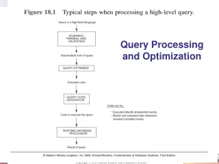
3. Basic Steps in Query Processing 1. Parsing and translation: translate the query into its internal form. This is then translated into relational algebra. Parser checks syntax, verifies relations. 2. Optimization: A relational algebra expression may have many equivalent expressions. Generation of an evaluation-plan. 3. Evaluation: The query-execution engine takes a query-evaluation plan, executes that plan, and returns the answers to the query

4. Query Processing : Optimization • A relational algebra expression may have many equivalent expressions E.g., balance2500(balance(account)) is equivalent tobalance(balance2500(account)) • Each relational algebra operation can be evaluated using one of several different algorithms E.g., can use an index on balance to find accounts with balance < 2500, or can perform complete relation scan and discard accounts with balance  2500 • Annotated expression specifying detailed evaluation strategy is called an evaluation-plan.

5. Basic Steps Query Optimization: Amongst all equivalent evaluation plans choose the one with lowest cost. • Cost is estimated using • Statistical information from the database catalog • e.g. number of tuples in each relation, size of tuples, number of distinct values for an attribute. • Statistics estimation for intermediate results to compute cost of complex expressions • Cost of individual operations • Selection Operation • Sorting • Join Operation • Other Operations How to optimize queries, that is, how to find an evaluation plan with “good” estimated cost ?

6. Evaluation plan branch = (branch_name, branch_city, assets) account = (account_number, branch_name, balance) depositor = (customer_id,customer_name, account_number) customer_name(branch_city=Brooklyn (branch (account depositor)))) A - customer_name ((branch_city=Brooklyn(branch)) (account depositor)) B - B A

7. Evaluation plan (cont.) • An evaluation plan defines exactly what algorithm is used for each operation, and how the execution of the operations is coordinated (e.g., pipeline, materialization).

8. Cost-based query optimization • Cost difference between evaluation plans for a query can be enormous • E.g. seconds vs. days in some cases • Steps in cost-based query optimization • Generate logically equivalent expressions using equivalence rules • Annotate resultant expressions to get alternative query plans • Choose the cheapest plan based on estimated cost

9. Generating Equivalent Expressions

10. Transformation of Relational Expressions • Two relational algebra expressions are said to be equivalent if the two expressions generate the same set of tuples on every legal database instance • Note: order of tuples is irrelevant • In SQL, inputs and outputs are multisets of tuples • Two expressions in the multiset version of the relational algebra are said to be equivalent if the two expressions generate the same multiset of tuples on every legal database instance. • An equivalence rule says that expressions of two forms are equivalent • Can replace expression of first form by second, or vice versa

11. Equivalence Rules 1. Conjunctive selection operations can be deconstructed into a sequence of individual selections. 2. Selection operations are commutative. 3. Only the last in a sequence of projection operations is needed, the others can be omitted. • Selections can be combined with Cartesian products and theta joins. • (E1X E2) = E1 E2 • 1(E12 E2) = E11 2E2 PL1 (PL2( … PLn (E))…)) = PL1(E)

12. Equivalence Rules (Cont.) 5. Theta-join operations (and natural joins) are commutative.E1  E2 = E2 E1 6. (a) Natural join operations are associative: (E1 E2) E3 = E1 (E2 E3)(b) Theta joins are associative in the following manner:(E1 1 E2) 2 3E3 = E1 1 3 (E22 E3) where 2involves attributes from only E2 and E3.

13. Pictorial Depiction of Equivalence Rules

14. Equivalence Rules (Cont.) 7. The selection operation distributes over the theta join operation under the following two conditions:(a) When all the attributes in 0 involve only the attributes of one of the expressions (E1) being joined.0E1  E2) = (0(E1))  E2 (b) When 1 involves only the attributes of E1 and2 involves only the attributes of E2. 1 E1 E2) = (1(E1))  ( (E2))

15. Õ = Õ Õ ( E E ) ( ( E )) ( ( E )) È q q L L 1 2 L 1 L 2 1 2 1 2 Equivalence Rules (Cont.) 8. The projection operation distributes over the theta join operation as follows: (a) if  involves only attributes from L1 L2: (b) Consider a join E1  E2. • Let L1 and L2 be sets of attributes from E1 and E2, respectively. • Let L3 be attributes of E1 that are involved in join condition , but are not in L1 L2, and • let L4 be attributes of E2 that are involved in join condition , but are not in L1 L2. Õ = Õ Õ Õ ( E E ) (( ( E )) ( ( E ))) È q È È È q L L 1 2 L L L L 1 L L 2 1 2 1 2 1 3 2 4

16. Equivalence Rules (Cont.) • The set operations union and intersection are commutative E1 E2 = E2 E1E1 E2 = E2 E1 • (set difference is not commutative). • Set union and intersection are associative. (E1 E2)  E3 = E1 (E2  E3)(E1 E2)  E3 = E1 (E2  E3) • The selection operation distributes over ,  and –. (E1 – E2) = (E1) – (E2)and similarly for  and  in place of –Also: (E1 – E2) = (E1) – E2 and similarly for in place of –, but not for  12. The projection operation distributes over union L(E1 E2) = (L(E1))  (L(E2))

17. Transformation: Pushing Selections down • Query: Find the names of all customers who have an account at some branch located in Brooklyn.customer_name(branch_city = “Brooklyn”(branch (account depositor))) • Transformation using rule 7a. customer_name((branch_city =“Brooklyn” (branch)) (account depositor)) • Performing the selection as early as possible reduces the size of the relation to be joined.

18. Example with Multiple Transformations • Query: Find the names of all customers with an account at a Brooklyn branch whose account balance is over $1000.customer_name((branch_city = “Brooklyn”  balance > 1000(branch (account depositor))) • Transformation using join associatively (Rule 6a):customer_name((branch_city = “Brooklyn”  balance > 1000(branch account)) depositor) • Second form provides an opportunity to apply the “perform selections early” rule, resulting in the subexpression branch_city = “Brooklyn”(branch)  balance > 1000 (account) • Thus a sequence of transformations can be useful

19. Multiple Transformations (Cont.)

20. Transformation: Pushing Projections down • When we compute (branch_city = “Brooklyn” (branch) account ) we obtain a relation whose schema is:(branch_name, branch_city, assets, account_number, balance) • Push projections using equivalence rules 8a and 8b; eliminate unneeded attributes from intermediate results to get:customer_name ((account_number( (branch_city = “Brooklyn” (branch) account )) depositor ) • Performing the projection as early as possible reduces the size of the relation to be joined. customer_name((branch_city = “Brooklyn”(branch) account) depositor)

21. Join Ordering Example • For all relations r1, r2, and r3, (r1r2) r3 = r1 (r2r3 ) (Join Associativity) • If r2r3 is quite large and r1r2 is small, we choose (r1r2) r3 so that we compute and store a smaller temporary relation.

22. Join Ordering Example (Cont.) • Consider the expression customer_name((branch_city = “Brooklyn” (branch)) (account depositor)) • Could compute account depositor first, and join result with branch_city = “Brooklyn” (branch)but account depositor is likely to be a large relation. • Only a small fraction of the bank’s customers are likely to have accounts in branches located in Brooklyn • it is better to compute branch_city = “Brooklyn” (branch) account first.

23. Measures of Query Cost

24. Measures of Query Cost • Cost is the total elapsed time for answering query • Many factors contribute to time cost • disk accesses, CPU, or even network communication • Typically disk access is the predominant cost, and is also relatively easy to estimate. Measured by taking into account • Number of seeks • Number of blocks read • Number of blocks written • Cost to write a block is greater than cost to read a block • data is read back after being written to ensure that the write was successful

25. Measures of Query Cost (Cont.) • In this course, for simplicity we just use the number of block transfersfrom disk as the cost measures (we ignore other costs for simplicity) • tT – time to transfer one block • we do not include cost to writing output of the query to disk in our cost formulae • Several algorithms can reduce disk IO by using extra buffer space • Amount of real memory available to buffer depends on other concurrent queries and OS processes, known only during execution • Required data may be buffer resident already, avoiding disk I/O • But hard to take into account for cost estimation

26. Cost of individual operationswe assume that the buffer can hold only a few blocks of data, approximately one block for each relationwe use the number of block transfers from disk as the cost measure we do not include cost to writing output of the query to disk in our cost formulae

27. Selection Operation File scan – search algorithms that locate and retrieve records in the file that fulfill a selection condition. • A1. Linear search. Scan each file block and test allrecords to see whether they satisfy the selection condition. • Cost estimate = br block transfers • br number of blocks containing records from relation r If selection is on a key attribute, can stop on finding record • cost = (br /2) block transfers Linear search can always be applied regardless of the ordering of the file and the selection condition. E.g., balance<2500(account) account file

28. Selection Operation (Cont.) E.g., branch-name=“Mianus”(account) • A2. Binary search. Applicable if selection is an equality comparison on the attribute on which file is ordered (sequentially ordered file on the attribute of the selection). • Assume that the blocks of a relation are stored contiguously • Cost estimate (number of disk blocks to be scanned): • cost of locating the first tuple by a binary search on the blocks • log2(br) • If there are multiple records satisfying selection • Add transfer cost of the number of blocks containing records that satisfy selection condition account file

29. Selections Using Indices E.g., balance<2500(account) - comparison • Index scan – search algorithms that use an index • selection condition must be on search-key of index. • A3. Primary index on candidate key, equality. Retrieve a single record that satisfies the corresponding equality condition • Cost = (hi+ 1) • A4. Primary index on non key, equality. Retrieve multiple records. • Records will be on consecutive blocks • Let b = number of blocks containing matching records Cost = (hi + b) • A5. Equality on search-key of secondary index. • Retrieve a single record if the search-key is a candidate key • Cost = (hi+ 1) • Retrieve multiple records if search-key is not a candidate key • each of n matching records may be on a different block • Cost = (hi+ n) • Can be very expensive! E.g.,  branch-name=“Mianus”(account)

30. Selections Involving Comparisons AV (r) or A  V(r) • By using • a linear file scan or binary search, • or by using indices in the following ways: • A6. Primary index, comparison. (Relation is sorted on A) • For A  V(r) use index to find first tuple  v and scan relationsequentially from there • For AV (r) just scan relation sequentially till first tuple > v; do not use index E.g.  branch-name >=“Mianus”(account) E.g.  branch-name <=“Mianus”(account)

31. Selections Involving Comparisons AV (r) or A  V(r) A.7 Secondary index, comparison. • For A  V(r) use index to find first index entry  v and scan index sequentially from there, to find pointers to records. • For AV (r) just scan leaf pages of index finding pointers to records, till first entry > v • In either case, retrieve records that are pointed to • requires an I/O for each record • Linear file scan may be cheaper E.g.  balance >=500(account) E.g.  balance <=500(account)

32. Implementation of Complex Selections Conjunction: 1 2. . . n(r) • Conjunctive selection using one index. • Select a combination of i and algorithms A1 through A7 that results in the least cost for i (r). • Test other conditions on tuple after fetching it into memory buffer. • Conjunctive selection using multiple-key index. • Use appropriate composite (multiple-key) index if available. • Conjunctive selection by intersection of identifiers, using more indices. • Use corresponding index for each condition, and take intersection of all the obtained sets of record pointers. • Then fetch records from file • If some conditions do not have appropriate indices, apply test in memory.

33. Algorithms for Complex Selections Disjunction:1 2 . . . n (r). • Disjunctive selection by union of identifiers. • Applicable if all conditions have available indices. • Otherwise use linear scan. • Use corresponding index for each condition, and take union of all the obtained sets of record pointers. • Then fetch records from file Negation: (r) • Use linear scan on file • If very few records satisfy , and an index is applicable to  • Find satisfying records using index and fetch from file

34. Sorting Sorting plays an important role in DBMS: 1) query can specify that the output be sorted 2) some operations can be implemented efficiently if the input relations are ordered (e.g., join) • We may build an index on the relation, and then use the index to read the relation in sorted order. Records are ordered logically rather than physically. May lead to one disk block access for each tuple.Sometimes is desirable to order the records physically • For relations that fit in memory, techniques like quicksort can be used. For relations that don’t fit in memory, external sort-merge is a good choice.

35. External Sort-Merge Sorting records in a file • Create sortedruns. Let i be 0 initially.Repeat (a) Read M blocks of relation into memory (b) Sort the in-memory blocks (c) Write sorted data to run file Ri; (d) increment i. until the end of the relation Let the final value of i be N Let Mdenote the number disk blocks whose contents can be buffered in main memory

36. External Sort-Merge (Cont.) • Merge the runs (N-way merge). We assume (for now) that N < M. • Use N blocks of memory to buffer input runs, and 1 block to buffer output. Read the first block of each run into its buffer page • repeat • Select the first record (in sort order) among all buffer pages • Write the record to the output buffer. If the output buffer is full write it to disk. • Delete the record from its input buffer page.If the buffer page becomes empty then read the next block (if any) of the run into the buffer. • until all input buffer pages are empty:

37. External Sort-Merge (Cont.) • If N M, several merge passes are required. • In each pass, contiguous groups of M - 1 runs are merged. • A pass reduces the number of runs by a factor of M -1, and creates runs longer by the same factor. • E.g. If M=11, and there are 90 runs, one pass reduces the number of runs to 9, each 10 times the size of the initial runs • Repeated passes are performed till all runs have been merged into one.

38. Example: External Sorting Using Sort-Merge M = 3 fr = 1 - tranfer 3 blocks- sort records - store in a run

39. External Merge Sort (Cont.) • Cost analysis: • Initial number of runs: br/M • Number of runs decrease of a factor M-1 in each merge pass.Total number of merge passes required: logM–1(br/M). • Block transfers for initial run creation as well as in each pass is 2br • for final pass, we don’t count write cost • we ignore final write cost for all operations since the output of an operation may be sent to the parent operation without being written to disk • Thus total number of block transfers for external sorting: 2br + 2brlogM–1(br / M) - br br ( 2 logM–1(br / M) + 1) ( - br because we do not include cost to writing output of the query to disk) In the example: 12( 2 log2 (12/ 3) + 1) = 12 (2*2 + 1) = 60 block transfers

40. Join Operation • Several different algorithms to implement joins • Nested-loop join • Block nested-loop join • Indexed nested-loop join • Merge-join • Hash-join • Choice based on cost estimate • Examples use the following information Customer: Number of records nc=10.000 Number of blocks bc=400 Depositor: Number of records nd=5.000 Number of blocksbd=100 customer = (customer_name, customer_street, customer_city, …) depositor = (customer_name,account_number,….) customer customer natural join customer customer.customer_iname = depositor.customer_iname depositor theta join

41. Nested-Loop Join r s • To compute the theta join rsfor each tuple tr in r do begin for each tuple tsin s do begintest pair (tr,ts) tosee if they satisfy the join condition  if they do, add tr• tsto the result.endend • r is called the outerrelation and s the inner relation of the join. • Requires no indices and can be used with any kind of join condition. • Expensive since it examines every pair of tuples in the two relations.

42. Nested-Loop Join (Cont.) • In the worst case, if there is enough memory only to hold one block of each relation, the estimated cost is nr bs + brblock transfers • If the smaller relation fits entirely in memory, use that as the inner relation. • Reduces cost to br + bsblock transfers • Assuming worst case memory availability cost estimate is • with depositor as outer relation: • 5000  400 + 100 = 2,000,100 block transfers, • with customer as the outer relation • 10000  100 + 400 = 1,000,400 block transfers • If smaller relation (depositor) fits entirely in memory, the cost estimate will be 500 block transfers. • Block nested-loops algorithm (next slide) is preferable. r s

43. Block Nested-Loop Join • Variant of nested-loop join in which every block of inner relation is paired with every block of outer relation. for each block Brofr do beginfor each block Bsof s do begin for each tuple trin Br do begin for each tuple tsin Bsdo beginCheck if (tr,ts) satisfy the join condition if they do, add tr• tsto the result.end end end end r s

44. Block Nested-Loop Join (Cont.) • Worst case estimate (if there is enough memory only to hold one block of each relation): br bs + br block transfers • Each block in the inner relation s is read once for each block in the outer relation (instead of once for each tuple in the outer relation • Best case (the smaller relation fits entirely in memory ):br+ bsblock transfers. • Improvements to nested loop and block nested loop algorithms: • Use index on inner relation if available (next slide)

45. Indexed Nested-Loop Join • Index lookups can replace file scans if • join is an equi-join or natural join and • an index is available on the inner relation’s join attribute • Can construct an index just to compute a join. • For each tuple trin the outer relation r, use the index to look up tuples in s that satisfy the join condition with tuple tr. • Worst case: buffer has space for only one block of r, and, for each tuple in r, we perform an index lookup on s. • Cost of the join: br+ nr c • Where c is the cost of traversing index and fetching all matching s tuples for one tuple or r • c can be estimated as cost of a single selection on s using the join condition. • If indices are available on join attributes of both r and s,use the relation with fewer tuples as the outer relation. index s r

46. Example of Nested-Loop Join Costs nc=10.000 bc=400 nd = 5000 bd=100 customer = (customer_name, customer_street, customer_city, …) depositor = (customer_name,account_number) • Compute depositor customer, with depositor as the outer relation. • Let customer have a primary B+-tree index on the join attribute customer-name, which contains 20 entries in each index node. • Since customer has 10,000 tuples, the height of the tree is  log20 10,000  = 4, and one more access is needed to find the actual data • depositor has 5000 tuples • Cost of block nested loops join • 400*100 + 100= 40,100 block transfers • assuming worst case memory • may be significantly less with more memory • Cost of indexed nested loops join • 100 + 5000 * 5 = 25,100 block transfers index depositor customer nd = 5000 bd=100 nc=10.000 bc=400

47. Merge-Join • Sort both relations on their join attribute (if not already sorted on the join attributes). • Merge the sorted relations to join them • Join step is similar to the merge stage of the sort-merge algorithm. • Main difference is handling of duplicate values in join attribute — every pair with same value on join attribute must be matched • Detailed algorithm in book

48. Merge-Join (Cont.) • Can be used onlyfor equi-joins and natural joins • Each block needs to be read only once (assuming all tuples for any given value of the join attributes fit in memory • Thus the cost of merge join is: br + bs block transfers • + the cost of sorting if relations are unsorted.

49. Hash-Join • Applicable onlyfor equi-joins and natural joins. • A hash function h is used to partition tuples of both relations • h maps JoinAttrs values to {0, 1, ..., n}, where JoinAttrs denotes the common attributes of r and s used in the natural join. • r0, r1, . . ., rn denote partitions of r tuples • Each tuple tr r is put in partition ri where i = h(tr[JoinAttrs]). • s0,, s1. . ., sn denotes partitions of s tuples • Each tuple tss is put in partition si, where i = h(ts[JoinAttrs]). • Note: In book, ri is denoted as Hri, si is denoted as Hsi and nis denoted as nh.

50. Hash-Join (Cont.)