Download
1 / 17
170 likes | 343 Views
Analytic Modeling of Load Balancing SCTP. Zhengliang Yi Tarek Saadawi, Myung Lee CUNY Graduate Center. Overview. SCTP, Stream Control Transmission Protocol (RFC2960). Multiple interfaces (possible multiple distinct multiple paths)

E N D
Analytic Modeling of Load Balancing SCTP Zhengliang Yi Tarek Saadawi, Myung Lee CUNY Graduate Center
Overview • SCTP, Stream Control Transmission Protocol (RFC2960). • Multiple interfaces (possible multiple distinct multiple paths) • Current specification: one primary path, others secondary paths to improve reachibility and reliability. • May be used as multiple path load balancing to dramatically improve throughput as well (current work).
Analytic Model of Standard SCTP-assumptions • Assumptions about the endpoints • Assuming sender is using SCTP congestion control mechanism defined by RFC2960. • Senders have unlimited amount of data to send so that all the flows can reach steady states. • Sender sends full-sized (fixed-sized) segments as fast as its congestion window allows. • Data are sent out via primary path and secondary paths only used for retransmission purpose.
Analytic Model of Standard SCTP-assumptions • Assumptions about network • Modeling SCTP behavior in terms of “rounds”, starts when the sender begins the transmission of a window of packets and ends when the sender receives first ACK for the packets in that window. “Round”=RTT • Assuming the time to send all packets in a window is smaller than the RTT. • Duration of a round (RTT) is independent of the window size. • Losses of one round are independent of the losses of any other rounds. Losses in one round is dependent: all packets in same round following a loss will be lost. Ideal of drop-tail queue, widely used on Internet
SCTP throughput model -Integrated Period Figure An integrated period. Method: Total number of packets transmitted Yi = YiTO+ YiSS + YiCA Length of integrated period i Zi = ZiTO+ ZiSS + ZiCA Throughputcan be expressed as B = E[Y] / E[S] Find average Y and Z for each period
Time-Out period ZTO • Retransmit lost packets via alternative path from slow start • E[YiTO] = E[RP] • E[RP] is the average number of lost packets when time-out happens. • Important in modeling SCTP because of its unique retransmission • Current size and position at cwnd • E[ZTO]= E[To] + E[TR] • E[To] is first time-out value • E[TR] is the average time for retransmitting all lost packets • W1 = 1 and γ = 1+1/b
Slow start period ZSS • Starts with one MSS • Increases cwnd by one MSS each ack. • Ends till encountering packet loss or ssthresh. E[W], average congestion window size in CA period.
Congestion avoidance period • E[ZCA] = E[n]E[ZQDP] • E[YCA] = E[n]E[YQDP] • E[n]: average number of QDPs in each CA • 1/ E[n]= Q: Given pkt loss(es), the probability that the packet loss(es) result in TO, not QDP (fast rtx process is triggered or not) .
Probability packet loss(es) result in TO, not QDP • Time out can only happen when packets get lost but fast retransmission can not be triggered, two situation: • Sender successfully sends out less than 4 packets in last round and following packets all lost • Sender successfully sends out 4 packets or more in last round but can only successfully sends out less than 4 packets in the round after. • Considering these two situations, we can find that: E[RP]: Ave No. of packets lost when time out happens.
Average congestion window size • Use above graph, we can easily find:
SCTP throughput model-throughput expression • Now we have everything we need
Simulation Environment • Using the NS2 network simulator • Drop-tail as the queuing scheme • Primary path for data, secondary path for retransmission
RTT of path1 to 20 ms, RTT of path2 to 50 ms and path 3 to 35ms. After 10 seconds, path3 is intentionally shut down
Our SCTP model compare with NS2 simulation Two lines are very close which indicates that our model can accurately predict the throughput of SCTP for a wide range of PER and RTT
DelAck with bytes oriented vs. acks oriented • Bytes oriented show significant throughput gain • Throughput gain decreases as PER increase. Reason: PER increase, CA decrease and TO increase. Two cwnd updating mechanisms act the same way during slow start, different during congestion avoidance. (RFC2960: max cwnd increase = 1 MSS)
Conclusions • Our analytic model precisely predicts steady state throughput of SCTP. • SCTP demonstrates better throughput compared with TCP, especially when packet error rate is high. • SCTP may be a better choice transport layer protocol for error prone networks such as wireless networks.