CS257 Query Optimization
CS257 Query Optimization. 2.4 An Algebraic Query Language. 2.4 An Algebraic Query Language. 2.4.1 Why Do We Need a Special Query Language? 2.4.2 What is an Algebra? 2.4.3 Overview of Relational Algebra 2.4.4 Set Operations on Relations 2.4.5 Projection 2.4.6 Selection

CS257 Query Optimization
E N D
Presentation Transcript
CS257 Query Optimization
2.4 An Algebraic Query Language 2.4.1 Why Do We Need a Special Query Language? 2.4.2 What is an Algebra? 2.4.3 Overview of Relational Algebra 2.4.4 Set Operations on Relations 2.4.5 Projection 2.4.6 Selection 2.4.7 Cartesian Product 2.4.8 Natural Joins 2.4.9 Theta-Joins 2.4.10 Combining Operations to Form Queries 2.4.11 Naming and Renaming 2.4.12 Relationships Among Operations 2.4.13 A Linear Notation for Algebraic Expressions 2.4.14 Exercises for Section 2.4
2.4.2 What is an Algebra? + - * / Projection Selection Natural Join Cartesian Product Union Intersect Minus
2.4.3 Overview of Relational Algebra Both numerical algebra and relational algebra are defined by (respective sets of) Algebraic Laws.
2.4.3 Overview of Relational Algebra Algebraic laws of Numbers that we have learned in calculus, algebra and etc since high school days
2.4.3 Overview of Relational Algebra Algebraic laws of relational algebra are “New” to most of us
2.4.3 Overview of Relational Algebra Special Relational Operators Projection Selection Natural Join Traditional Set Operators 4. Cartesian Product 5. Union 6. Intersect 7. Minus
QUERY OPTIMIZATION In query optimization the query is transformed by compiler into such a form that can solve the problem “fastest ”
QUERY OPTIMIZATION Illustration: 2 * 3 + 5 * 3 From the laws of Numerical algebra, it can be computed as follows:. Method I - It computes in three operations 2 * 3 + 5 * 3 = 6 (first) + 15(second) = 21 (third)
QUERY OPTIMIZATION Illustration: 2 * 3 + 5 * 3 From the laws of Numerical algebra, it can Also be computed as follows:. Method II- transform into equivalent one. = (2 + 5) * 3 = 7 (first) * 3 = 21 (second) It computes in two operations So compiler choose Method II
Roles of Relational Algebra QUERY OPTIMIZATION Similar Idea is used in Relational Algebra So we need to know the Algebraic Laws of Relational Algebra well That is the main goal for Ch5 and part of Ch16
2.4.4 Set Operations on Relations Recall Venn Diagram Y X b c d e a
Query Algebra In DBMS a query is turn into a sequence of operators on U • Theseoperators forms the query algebra (Extended RA)
Query Algebra Bag operations: RSSUM(# of times in R, - - - - - - S) R∩S Min (# of times in R, - - - - - - S)
Examples Two bags: R = {A, B, B} S = {C, A, B, C} R S ={A, A, B, B, B, C, C} R ∩ S = {A, B} R—S ={B} (Obvious?)
Selection: C(R) SQL: Select * from R where C C can involve computable formulas
Projection: L(R) Select L from R
Projection: L(R) • L can have : 1. A single attribute of R. 2. An expression x y: It means we take the attribute x of R and rename it as y. 3. An expression E z where E is an expression involving attributes of R and z is a new name for the attribute that results from the calculation . Ex: a+b x
Theta Join: Theta Join: R c S = σc(RS) Natural Join (Special Case of Theta Join) R cS = πL(σc(RS)) Where L: The list that meets the condition c of equality and redundant attributes are dropped
SORTING OPERATOR () • This is the SQL ORDER BY clause and denoted by the operator L (R) • where R is a relation and L a list of some of R’s attributes in the relation R but with the tuples of R sorted in the order indicated by L. • If L is a1, a2…an, then tuples are first sorted by a1, then a2 until an. By default sorting is in ascending order.
Grouping andAggregation: L(R) Select L(=A,B) from R group by A A: aggregating attribute B: aggregated attributes
Grouping andAggregation: L(R) It returns a relation that partitions the tuples of R in to groups. Each group consists of all tuples having one particular assignment of values to the grouping attributes A in L. L also contains B, Aggregated attributes, in the form: Aggregation operator Name
Grouping and Aggregation • Aggregation operators : AVG, SUM, COUNT, MIN, MAX • Grouping: GROUP BY clause in SQL • Having clause must follow a GROUP BY clause
Grouping and Aggregation • Grouping and aggregation are generally implemented together. So we have a single operator defining it • It is a generalized Projection Operator • Delicate-elimination operator is a special Aggregation operator.
pnum, sum(qty)sum(SP) Select pnum, sum(qty) as sum from SP group by pnum;
Some rules on selection: 1.σc1 and c2(R) = σc1(σc2 (R) ) 2.σc1 or c2(R) = (σc1R) s (σc2 R) whenever c apply to R or S
Some Rules about Selection: 3.σc(R S) = (σcR ) (σc S) 4.σc(R S) = (σcR) (σc S) 5.σc(R S) = (σcR) (σcS) whenever c apply to R or S
Rules about (generalized) Projection: 6. We may introduce a (generalized) projection anywhere in an expression tree, as long as it eliminates only attributes that are never used by any operator above
Some Rules about Projection: 7. L(R c S) =L(M(R)cN(R)) 8. L(R S) =L(R)L(S)
Query Optimization Example Select p.pname, p.pnum, sum(sp.qty) as sum from Parts p, Shipments sp where p.pnum = sp.pnum and p.weight > 10 group by p.pname, p.pnum having sum(sp.qty) >= 200;
Translating to Query Algebra Step 1 (P SP) Step 2σP.PNUM = SP.PNUM and P.WEIGHT >10(PSP) = Step 3σSUM >= 200(γP.PNAME, P. PNUM, SUM(SP.QTY) → SUM ())=, Step 4 πP.PNAME, P. PNUM, SUM() =
πP.PNAME, P. PNUM, SUM σSUM >= 200 γP.PNAME, P. PNUM, SUM(SP.QTY) → SUM σP.PNUM = SP.PNUM and P.WEIGHT >10 P SP
Computing in QA = πP.PNAME, P. PNUM, SUM( γP.PNAME, P. PNUM, SUM(SP.QTY) → SUM ( σP.WEIGHT >10 and P.PNUM = SP.PNUM (PSP)) =(1)πP.PNAME, P. PNUM, SUM( γP.PNAME, P. PNUM, SUM(SP.QTY) → SUM ( σP.WEIGHT >10 (σP.PNUM = SP.PNUM (PSP) )
Computing in QA πP.PNAME, P. PNUM, SUM( γP.PNAME, P. PNUM, SUM(SP.QTY) → SUM( σP.WEIGHT >10(σP.PNUM = SP.PNUM (PSP) )=(6) πP.PNAME, P. PNUM, SUM( γP.PNAME, P. PNUM, SUM(SP.QTY) → SUM ( σP.WEIGHT >10 (πLσP.PNUM = SP.PNUM(PSP) )
Computing in QA πP.PNAME, P. PNUM, SUM( γP.PNAME, P. PNUM, SUM(SP.QTY) → SUM ( σP.WEIGHT >10 (πLσP.PNUM = SP.PNUM(PSP) )=D πP.PNAME, P. PNUM, SUM( γP.PNAME, P. PNUM, SUM(SP.QTY) → SUM (σP.WEIGHT >10(PP.PNUM = SP.PNUM SP )
Computing in QA πP.PNAME, P. PNUM, SUM( γP.PNAME, P. PNUM, SUM(SP.QTY) → SUM (σP.WEIGHT >10(PP.PNUM = SP.PNUM SP )=(5) πP.PNAME, P. PNUM, SUM( γP.PNAME, P. PNUM, SUM(SP.QTY) → SUM ( σP.WEIGHT >10(P)P.PNUM = SP.PNUM σP.WEIGHT >10(SP) )
Computing in QA πP.PNAME, P. PNUM, SUM ( γP.PNAME, P. PNUM, SUM(SP.QTY) → SUM ( (σP.WEIGHT >10(P)P.PNUM = SP.PNUMσP.WEIGHT >10(SP) ) =D πP.PNAME, P. PNUM, SUM( γP.PNAME, P. PNUM, SUM(SP.QTY) → SUM ( σP.WEIGHT >10(P)P.PNUM = SP.PNUM(σP.WEIGHT >10=1)(SP) )=
Final Expression = πP.PNAME, P. PNUM, SUM( σSUM >= 200(γP.PNAME, P. PNUM, SUM(SP.QTY) → SUM ( σP.WEIGHT >10(P)P.PNUM = SP.PNUM(SP) )=
πP.PNAME, P. PNUM, SUM σSUM >= 200 γP.PNAME, P. PNUM, SUM(SP.QTY) → SUM P.PNUM = SP.PNUM σp.weight SP P
Final Expression is computationally cheaperthan σP.WEIGHT >10(P) is smaller than P
πP.PNAME, P. PNUM, SUM σSUM >= 200 P.PNUM = SP.PNUM σp.weight γP. PNUM, SUM(SP.QTY) → SUM SP P
πP.PNAME, P. PNUM, SUM P.PNUM = SP.PNUM σp.weight σSUM >= 200 P γP. PNUM, SUM(SP.QTY) → SUM SP
EXPRESSION TREES • Generated by combining several Qerry Algebra operators into one expression by applying one operator to the result(s) of one or more operators. • The leaves of this tree are names of relations. Interior nodes are operators, which are applied to the relations represented by its child or children

