Optimizing SQL Queries: Understanding SARGability and Index Selection
Query optimization is essential for improving SQL performance. This involves analyzing SQL statements, focusing on WHERE clauses, and identifying SARGable predicates that enable index usage. SARG (Search ARGuments) predicates include operators like =, >, and ranges. Non-SARGable predicates, like NOT or !=, hinder performance. The optimizer assesses index usability based on selectivity and logical reads. Understanding index statistics, including density and step values, aids in selecting the most efficient query execution path, balancing cost against speed for optimal performance.

Optimizing SQL Queries: Understanding SARGability and Index Selection
E N D
Presentation Transcript
Query Optimization • Query Analysis • Index Selection • Costing
Query Analysis • Evaluates the SQL statement • Looks closely at the WHERE clauses • Determines SARG predicates
SARG predicates • Search ARGuments • A SARG contains a constant expression or a variable that resolves to an constant that acts on a column • The importance of an SARGable predicate is that an index might be used to resolve it
Types of SARG Predicates • = • > • < • => • <= • Between • sometimes Like • ‘A%’ is SARGable • ‘%A’ is not SARGable
Non-SARGable Predicates • NOT • != • <> • !> • !< • NOT EXISTS • NOT IN • NOT LIKE
Changing to SARGable Predicates • Recognize these are the same • !> -- <= • !< -- >= • Think about how to state the equality without using a not
Index Selection • The optimizer determines whether an index exists for a SARGable clause, assesses the index's usefulness in determining selectivity of the clause estimates the cost to find qualifying rows • After the optimizer finds a potentially useful index, it evaluate the index based on the selectivity or density of the clause
Index Statistics • Index Statistics are stored in the catalog (sysindexes) for each index • The statistics are stored as a histogram and consists of even sampling of values for the index key (or the first column of the index) • This information includes: • Density • Step Values
Density • Is a ratio of the number of distinct keys for an index to the number of rows in the table • For example if a table has 8345 rows • A unique index has one index entry for each row with an density of 1/8345 or 0.0012 • For a nonunique index with a density of 0.21265 each index key would point to 1807
Logical Reads • Logical Reads or data page accesses are what are needed to retrieve the rows from a data page • In our example assume there are about 40 rows per page, or about 209 total pages • The chances of two adjacent index entries pointing to the same page is about 0.5% (1 in 209) • Using our non unique index that means that we would probably do 1807 logical reads to use this index, plus whatever was needed for the index itself • It would be faster to scan the table
Step Values • Density assumes a smooth distribution of data • One key would not return a significant larger number of rows than another • Step values account for this skewing of data • It keeps count of actual number of rows for the most popular key values
Density Calculation • NF is NonFrequent values – then number of values that appear no more than once in the histogram step values • = (NF count/distinct NF count)/number of rows • Density is equal to a value of 0 – 1 • Density * the number of rows in a table will give an estimation of the number of rows returned by a single value in an index
Density versus All_Density • Densities are calculated in two different ways • The first is calculated for all columns of the index (density) • The second is calculated for all combinations of columns of the index (all_density)
Setup for Density Example • If we build an index on tblClassSection on Instructor_id, Class_id, Section_id • Then run the following command: • Dbcc show_statistics (tblClassSection, testidx) • We receive the following results
Statistics Results Updated Rows Rows Sampled Steps Density Avg Key Len May 16 2002 9:09AM 35 35 7 0.0 8.0 All Density Avg Len Columns 0.14285715 2.0 Instructor_ID 4.5454547E-2 7.0 Instructor_ID, Class_ID 2.8571429E-2 8.0 Instructor_ID, Class_ID, Section_ID
Steps Results Range Hi Key Range Rows Eq Rows Distinct Avg 11 0.0 4.0 0 0.0 13 0.0 1.0 0 0.0 14 0.0 5.0 0 0.0 16 0.0 4.0 0 0.0 17 0.0 1.0 0 0.0 18 0.0 7.0 0 0.0 19 0.0 13.0 0 0.0
Costing • Even if an index is useful, it might not be the cheapest path • Multiple indexes might be available • Cost is driven by the estimated logical I/O • Each index is evaluated on the number of likely 'hits' based on density and step values in statistics.
Cost Evaluation • Based on these values the optimizer determines the likely number rows that would qualify for a given SARG. • It might find multiple indexes that can find qualifying rows. • It might determine that scanning the table and checking every row is best. • It will chose the access method that predicts the fewest logical reads. • Estimated logical reads for different access methods
Cost Formulas • Table Scan • Clustered Index • Non Clustered Index on a heap • Nonclustered Index on a table with a clustered index • Covering nonclustered index
Table Scan • The total number of data pages
Clustered Index • The number of levels in the index plus the number of data pages to scan. Data pages to be scanned = nunber of qualifying rows / rows per data page.
Non Clustered Index on a heap • The number of levels in the index plus the number of leaf pages plus the number of qualifying rows.
Nonclustered Index on a table with a clustered index • The number of levels in the index plus the number of leaf pages plus the number of qualifying rows times the cost searching for a clustered index key.
Covering nonclustered index • The number of levels in the index plus the number of leaf index pages (qualifying rows / rows per leaf page). • The data page need not be accessed because all necessary information is in the index key.
Multiple Index Scan • SQL Server will use more than one index to resolve a query. • The cost formula changes. • In addition to the cost for each index, there is additional cost for finding the intersection of the indexes. • Each index contains a locator for actual data, the results of the tow index searches are treated as work tables and joined together on locator data to find the rows that satisfy both indexes.
Joins • Nested Loop Joins • Merge Joins • Hash Joins
DEPARTMENT Dept_no Manager 2 Laszio 5 Wehland 6 Graeffe 8 Waymire 10 Aebi 13 Soukup 15 Berensen EMPLOYEE ID Name Dept_no 1 Pike 2 2 Delaney 6 3 Harvey 7 4 Moran 10 5 Rogerson 14 6 Karaszi 13 7 Fields 11 8 Robertson 4 9 Pfeiff 1 10 Hotz 7 11 Dwyer 2 12 Talmadge 12 Join Example Tables
Nested Loop Join • A set of nested iterations • A row is found in the first (outer) table then the second (inner table is searched for that value) • The simplest join • Good for small joins, bad for large joins
Nested Loop Psuedocode Where dept.deptno = empl.deptno Do (until no more dept rows); GET NEXT dept row; begin Scan empl, get next empl row for dept end
Merge Join • The two tables are sorted on the common (join) key • The two tables are then worked together to find common values. • Most often the two tables will require a common index • SQL Server may choose to actually sort the tables if the clustered indexes do not exist. • Generally faster than Nested Loop for larger tables
Merge Join Psuedocode Where dept.deptno = empl.deptno GET on dept row and one empl row DO (until one input is empty); IF dept_no values are equal Return values from both rows ELSE IF empl.dept_no < dept.dept_on GET new empl row ELSE GET new dept row Get NEXT dept row END
Hash Join • May be used where no useful index exists • Hashing lets you determine whether a particular data item matches an already existing value by dividing the existing data into groups based on some property. You put all the data with the same value in what we can call a hash bucket. Then to see if a new value has a match in existing data, you simply look in the bucket for the right value. • SQL Server builds these hash buckets from the values of one table (called the build input). It then takes the second table (called the probe input) to see if the hash values exist for it • Hash Joins are quite expensive in terms of memory
Hash Join Psuedocode Allocate an Empty Hash Table For Each Row in the Build Table Determine hash bucket and insert relevant columns For Each Row in the Probe Table Determine hash bucket and scan for matches Deallocate Hash Table
Other Clauses • Group By/Order By/Distinct • Generally, SQL Server does a sort to satisfy a Group By, Order By or Distinct clauses • If the right index exists, SQL Server will attempt to use this index for the query (avoiding the sort)
Group By vs Order By • If SQL Server uses a sort or an index to resolve a Group By, the answer set will come back in Group By order, unless an Order By overrides it • SQL Server may also chose to use a hashing algorithm to resolve a Group By in which case the Group By would come back in an unpredictable order • If you want your answer set in a specific order, use the Order By clause
Monitoring Query Performance • STATISTICS IO • STATISTICS TIME • Showplan
STATISTICS IO • Set Statistics IO ON • Logical Reads • Physical Reads • Read Ahead Reads • Scan Counts
STATISTICS TIME • Set Statistics Time ON • Shows the elapsed and CPU times required to process the query
SHOWPLAN • Examines execution plan for a query • For Text • Set showplan_text on • Set showplan_all on • For Graphical • Use Display Extimated Execution Plan from Query Menu

