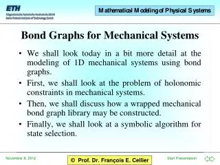
Bond Graphs for Mechanical Systems
We shall look today in a bit more detail at the modeling of 1D mechanical systems using bond graphs. First, we shall look at the problem of holonomic constraints in mechanical systems. Then, we shall discuss how a wrapped mechanical bond graph library may be constructed.

Bond Graphs for Mechanical Systems
E N D
Presentation Transcript
We shall look today in a bit more detail at the modeling of 1D mechanical systems using bond graphs. First, we shall look at the problem of holonomic constraints in mechanical systems. Then, we shall discuss how a wrapped mechanical bond graph library may be constructed. Finally, we shall look at a symbolic algorithm for state selection. Bond Graphs for Mechanical Systems
State variables in mechanical systems Holonomic constraints Wrapping mechanical bond graph models State selection Initial conditions Protected variables An example State selection algorithm Table of Contents
We have already seen that masses (inertias) can be modeled using bond graph inductors, whereas springs can be modeled using bond graph capacitors. Hence the natural state variables in a bond graph description of a mechanical system are the absolute (angular) velocities of the bodies and the spring forces (torques). In a model of a mechanical system described in this fashion, the (angular) positions are missing. They are not needed for a proper and complete description of the dynamics of the system. State Variables in Mechanical Systems
This causes problems, as it is relevant to know whether two bodies occupy the same space at the same time, i.e., whether they bump into each other or not. Also, when two bodies are connected at a point (e.g. through a joint), it is insufficient to state that the velocities of these points are equal. It should be stated that their positions are identical. Such positional constraints are being referred to as holonomic constraints in the mechanical literature. The corresponding velocity constraints (non-holonomic constraints) don’t need to be specified separately, because they can be derived automatically from the holonomic constraints. Holonomic Constraints
For this reason, it may be better to find an alternate description that uses the absolute velocities and positions of bodies as state variables, leaving the spring forces out. Can this be done within the framework of the bond graph methodology? It can, and this is how the two wrapped 1D mechanical bond graph libraries (for translational and rotational motions) have been built. Holonomic Constraints II
We introduce two translational flange connectors. These are similar to those of the standard library, but they are not identical, as they shall contain a second across variable: the velocity, v. Hence our mechanical models will be incompatible with those of the standard library. The two flange models are actually identical. They are both offered for optical reasons only. The Mechanical Connectors
We also need a real signal connector. This is similar to the input and output connectors of the blocks library, but the signal is bidirectional, rather than being unidirectional. The Mechanical Connectors II
We need wrapper models that convert the mechanical connectors to bond graph connectors and back. Since the bond graph connector cannot include the positional information, this must be separated out into a second signal connector. The Wrapper Models
Since the mechanical connector corresponds to a mechanical node, i.e., a point where the sum of all forces (torques) adds up to zero, it corresponds to a bond graph 1-junction, rather than to a bond graph 0-junction. Consequently, it is here the effort variable that must get the negative sign. The Wrapper Models II
We are now ready to look at the model of a sliding mass. The Sliding Mass Model The two state variables are the f variable of the inductor model and the output of the internal integrator of the q sensor.
The model is split into an upper (bond graph) part that deals with velocities and forces, and a lower (signal) part that deals with positional information. The position s calculated by the sensor is the position of the center of the mass bar. The position of the left connector is L/2 to the left of the center, and the position of the right connector is L/2 to the right of the center. These positional values are distributed out to the left and to the right through the mechanical connectors bond graph model (v,f) signal graph model (s) The Sliding Mass Model II
The natural state variables of this model are the internal variables I.f and sAbs.Integrator1.y. This is inconvenient. The user of the model would prefer to use the local variables v and s of the mass model as state variables. Dymola can be told to modify the equations such that, if possible, the desired variables are being used as state variables, i.e., show up in the simulation code with a der() operator. We shall discuss later in this lecture, how this can actually be accomplished. The Sliding Mass Model III
One question that remains is, for which variables we now have to specify the initial conditions. Do we do it for the new state variables s and v, or do we still do it for the natural state variables? It turns out that we can do either or, but not both. Dymola will use the specified values as start values of an iteration and iterate on the unknown initial values of the new state variables, until it finds a set of initial conditions that is consistent with the information that has been specified by the user. The Sliding Mass Model IV
We are now ready to look at the model of a spring. The Spring Model The spring is modeled as a modulated effort source, i.e., without an integrator of its own. It imports the positional information through its two terminals.
The spring can be either described using the equation: or using the differentiated form: Until now, we always used the latter representation, i.e., a capacitor, whereas now, we are using the former equation. Both work equally well, in principle. The Spring Model II fx = k · (xleft – xright ) dfx/dt = k · (vleft – vright )
There is however a problem. The new spring model imports the needed positional information through its two terminals. Since positional information is only computed by masses and inertial frames, this spring model can only be placed either between two masses or between a mass and the ground. In particular, it is not possible to place a spring and a damper in series with each other. The Spring Model III (Placing two springs in series would have worked correctly if we had used a-causal models for signal processing rather than relying on the causal blocks from the block library.)
The former model (using a capacitor) did not share this limitation. Hence our new spring model is a bit of a dirty trick. … the same dirty trick by the way that the standard library is using, albeit without offering a bond graph interpretation. The Spring Model IV
The equation layer doesn’t offer any surprises. The relative position and velocity of the spring are calculated here, since these are variables that the user may like to display. The Spring Model V The remaining models of the library are what we would expect them to be, thus they don’t need to be discussed here.
Let’s now look at the expanded view of the equation layer of the spring model. I manually placed the keyword protected in front of the declarations of variables to the inside of the wrapper models. The effect of this measure is to prevent these variables from being displayed in the simulation window. In this way, the model parameters will look exactly the same in the simulation window as using the corresponding model of the standard library. The model has been wrapped tightly. Wrapping Tightly – Protected Variables
Given the following mechanical system: An Example
Using the translational sub-library of the mechanics library of the BondLib library, this system can be modeled as follows: An Example II
The initial conditions were calculated correctly. Due to information hiding (protected variables), only those variables external to the wrapper models are visible. An Example III
Until now, we have always used the “capacitor” voltages and “inductor” currents of our bond graph models as our state variables. Sometimes, this is not desirable. We may have specific wishes as to which variables should be used as state variables. In some cases (as we shall see later), the choice of state variables also influences the run-time efficiency of the generated simulation code. The number of generated equations may depend heavily on a wise choice of state variables. The Selection of State Variables
Dymola supports the concept of selecting state variables differently from those that the system would normally choose. To this end, the user declares a desired state variable as follows: Dymola complies with the request by means of a variant of the Pantelides algorithm. The Selection of State Variables II Real x(stateSelect = StateSelect.prefer)
If the desired state variable already appears in differentiated form, use it whenever possible as a state. If the desired state variable does not already appear in differentiated form, differentiate the equation that computes the desired state, add it to the set of equations, and create a new integrator for it. We now have one equation too many. If in the process of differentiation additional algebraic variables are being differentiated, differentiate the equations defining those variables as well, add them also to the set of equations, but don’t add new integrators for them. The Selection of State Variables III
In the process of these additional differentiations, new variables and new equations are added to the set, so that at the end of the process, there is still one equation too many. If the desired state variable is legitimate, at least one of the previous state variables occurs among the set of equations that were differentiated. Throw the integrator associated with one of those state variables away to once again end up with an identical number of equations and unknowns. The Selection of State Variables IV
Given our “standard” electrical circuit. We have already learnt how to retrieve a causal set of equations from it. 1:U0 = f(t) 2:v2 = uC 3:uR2 = uC 4:uL = U0 5:v1 = U0 6:iR2 = uR2 / R2 7:uR1 = v1 – v2 8:iR1 = uR1 / R1 9:iC = iR1 – iR2 10:i0 = iL + iR1 11:diL/dt = uL / L1 12:duC/dt = iC / C1 The Selection of State Variables V
We wish to derive a different set of simulation equations that uses uR1 as a state variable, while eliminating one of the two former state variables from the set. To this end, we manually implement the state selection algorithm described earlier. The Selection of State Variables VI
Continue with this equation. 1:U0 = f(t) 2:v2 = uC 3:uR2 = uC 4:uL = U0 5:v1 = U0 6:iR2 = uR2 / R2 7:uR1 = v1 – v2 8:iR1 = uR1 / R1 9:iC = iR1 – iR2 10:i0 = iL + iR1 11:diL/dt = uL / L1 12:duC/dt = iC / C1 dv1 = dU0 Now differentiate these two equations. dv2 = duC Differentiate this equation, while creating a new derivative for uR1, but no new derivatives for v1 and v2. Eliminate this integrator. The Selection of State Variables VII duR1/dt = dv1 – dv2 dU0 = df(t)/dt
We can now apply the Tarjan algorithm to the new set of equations. duR1/dt = dv1 – dv2 duR1/dt = dv1 – dv2 1:U0 = f(t) 2: v2 = uC 3: uR2 = uC 4: uL = U0 5: v1 = U0 6: iR2 = uR2 / R2 7:uR1 = v1 – v2 8: iR1 = uR1 / R1 9: iC = iR1 – iR2 10: i0 = iL + iR1 11: diL/dt = uL / L1 12: duC = iC / C1 1:U0= f(t) 2: v2 = uC 3: uR2 = uC 4: uL = U0 5: v1 = U0 6: iR2 = uR2 / R2 7:uR1 = v1 – v2 8:iR1 = uR1 / R1 9: iC = iR1 – iR2 10: i0 = iL + iR1 11: diL/dt = uL / L1 12: duC = iC / C1 dv1 = dU0 dv1 = dU0 dv2 = duC dv2 = duC dU0 = df(t)/dt dU0 = df(t)/dt The Selection of State Variables VIII
duR1/dt = dv1 – dv2 duR1/dt = dv1 – dv2 1:U0= f(t) 2: v2 = uC 3: uR2 = uC 4:uL = U0 5:v1 = U0 6: iR2 = uR2 / R2 7:uR1 = v1 – v2 8:iR1 = uR1 / R1 9: iC = iR1 – iR2 10:i0 = iL + iR1 11: diL/dt = uL/ L1 12: duC = iC / C1 1:U0= f(t) 2: v2 = uC 3: uR2 = uC 4: uL = U0 5: v1 = U0 6: iR2 = uR2 / R2 7:uR1 = v1 – v2 8:iR1 = uR1 / R1 9: iC = iR1 – iR2 10: i0 = iL + iR1 11: diL/dt = uL / L1 12: duC = iC / C1 dv1 = dU0 dv1 = dU0 dv2 = duC dv2 = duC dU0 = df(t)/dt dU0 = df(t)/dt The Selection of State Variables IX
duR1/dt = dv1 – dv2 duR1/dt = dv1 – dv2 1:U0= f(t) 2:v2 = uC 3: uR2 = uC 4:uL = U0 5:v1 = U0 6: iR2 = uR2 / R2 7:uR1 = v1 – v2 8:iR1 = uR1 / R1 9: iC = iR1 – iR2 10:i0 = iL + iR1 11:diL/dt = uL/ L1 12: duC = iC / C1 1:U0= f(t) 2: v2 = uC 3: uR2 = uC 4:uL = U0 5:v1 = U0 6: iR2 = uR2 / R2 7:uR1 = v1 – v2 8:iR1 = uR1 / R1 9: iC = iR1 – iR2 10:i0 = iL + iR1 11: diL/dt = uL/ L1 12: duC = iC / C1 dv1 = dU0 dv1 = dU0 dv2 = duC dv2 = duC dU0 = df(t)/dt dU0 = df(t)/dt The Selection of State Variables X
duR1/dt = dv1 – dv2 duR1/dt = dv1 – dv2 1:U0= f(t) 2:v2 = uC 3:uR2 = uC 4:uL = U0 5:v1 = U0 6:iR2 = uR2 / R2 7:uR1 = v1 – v2 8:iR1 = uR1 / R1 9:iC = iR1 – iR2 10:i0 = iL + iR1 11:diL/dt = uL/ L1 12:duC = iC/ C1 1:U0= f(t) 2:v2 = uC 3: uR2 = uC 4:uL = U0 5:v1 = U0 6: iR2 = uR2 / R2 7:uR1 = v1 – v2 8:iR1 = uR1 / R1 9: iC = iR1 – iR2 10:i0 = iL + iR1 11:diL/dt = uL/ L1 12: duC = iC / C1 dv1 = dU0 dv1 = dU0 dv2 = duC dv2 = duC dU0 = df(t)/dt dU0 = df(t)/dt The Selection of State Variables XI
We ended up with 16 equations in 16 unknowns instead of the former 12 equations in 12 unknowns. This solution is a bit less run-time efficient. However, the variables that now appear differentiated in the model are the inductor current, iL, and the resistive voltage, uR1. duR1/dt = dv1 – dv2 1:U0= f(t) 2:v2 = uC 3:uR2 = uC 4:uL = U0 5:v1 = U0 6:iR2 = uR2 / R2 7:uR1 = v1 – v2 8:iR1 = uR1 / R1 9:iC = iR1 – iR2 10:i0 = iL + iR1 11:diL/dt = uL/ L1 12:duC = iC/ C1 dv1 = dU0 dv2 = duC dU0 = df(t)/dt The Selection of State Variables XII