Modeling Multi-Element Systems Using Bond Graphs
Explore the fundamentals of multi-element systems modeling with real bond graphs, focusing on mixture properties, transport phenomena, and a detailed model of a pressure cooker. Understand the advantages and disadvantages of complex CF-elements in thermodynamics.

Modeling Multi-Element Systems Using Bond Graphs
E N D
Presentation Transcript
Modeling Multi-Element SystemsUsing Bond Graphs 18.10.2001 Modeling Multi-ElementSystems Using Bond Graphs Jürgen Greifeneder François E. Cellier Jürgen Greifeneder, François Cellier
Jürgen Greifeneder: Review on paper the main aspects of paper 1 and 2 Pressure Cooker already diskussed in 2, however, only in a really short way, as the model is based on the multi-element system theory also. Contents • Introduction • Review • Basics of Multi-Element Systems • Mixture Properties • Transport Phenomena • Model of a Pressure Cooker • Conclusions Jürgen Greifeneder, François Cellier
} Introduction • Describing a thermodynamical problem necessitates 3 variables. • Separation in storage and dissipative elements. • Storage elements calculate the potentials and therefore need to know about the matter, they are representing. Dissipative elements calculate flows and do not care, which matter they are dealing with (network theory). • Elements do not know about each other. • No quasi-stationary or flow-equilibrium assumptions were made. • Contrary to earlier efforts in this field, this work delt with real, rather than pseudo bond graphs. Jürgen Greifeneder, François Cellier
Jürgen Greifeneder: 3 storage elements, but none of them can calculate its potential on ist own Bus- vs. Vektorbond } The C-field (storage element) Icon: CF 3 Ø 0 . S T C CF C C g q . M p 0 0 Jürgen Greifeneder, François Cellier
Jürgen Greifeneder: Unterscheidung zwischen RF-Element und RF-Konzept !!! Hinweis, daß es sich um Dichte und spezifische Entropie handelt } Basic dissipative Elements 3 3 CD CF CF 2 1 3 3 DVA Volume work: CF CF 2 1 r r , s , s Convection: 1 1 2 2 CF CF 2 1 3 3 Ø 3 3 Ø RF Conduction: Jürgen Greifeneder, François Cellier
Jürgen Greifeneder: • Advantages of n+2-CF-Element: • no constraint equations • topological model of a complex system would be simpler and more easy to understand • Disadvantages • The previously introduced structures would have to be extended • ?Internal equations of the C-field would change in accordance with the composition of the mixture • unnecessary complexity, especially in the case of simple systems • Processes would be hidden, that the authors would like to make visible • However, as this is the classical thermodynamical approach, one would certainly have done so also } Traditional Thermodynamics CF ? .... 0 0 0 0 Ø 1 2 3 n .... g2 g1 . . . . Mn g3 M3 M2 M1 gn C n CF C C q T . S p 0 0 One Temperature, one pressure and n partial mass’ => n+2 equations. Jürgen Greifeneder, François Cellier
Jürgen Greifeneder: Each matter has its own CF-Element. Each CF-Element is assumed to be a direct neighbor of each other element The contact surfaces between the different matters are assumed to be infinitely large => temperature and pressure may equilibrate infinitely fast. However, the corresponding transfer rates cannot be chosen infinitely large and therefore, the temperature and the pressure of the different components can assume somewhat different values (in the simulation). Although, if let alone, the will equilibrate, eventually. } CF CF 1 2 Multi-Element Mono-Phase Systems DVA CD 2 2 3 3 Ø Ø 2 2 CF 3 DVA CD DVA CD 3 2 2 Ø Jürgen Greifeneder, François Cellier
Jürgen Greifeneder: Ideally mixed = molecules are distributed at random (prediction, which molecul becomes a neighbor of which other molecules is not possible CF CF {M1} {M2} MI 2 {x1} {x2} 1 } Ideal and Non-Ideal Mixtures • In the process of mixing, additionally entropy will be created, which must be distributed among the participating components • Distribution is a function of the molar fractions • CF-Elements are not supposed to know about each other • Þonly necessary information will be provided Jürgen Greifeneder, François Cellier
Jürgen Greifeneder: Non-Ideal Mixtures: Volume will change also; specific excess volume and entropy of a non-ideal mixture are tabulated in the literature CF 2 } Ideal and Non-Ideal Mixtures • In the process of mixing, additionally entropy will be created, which must be distributed among the participating components • Distribution is a function of the molar fractions • CF-Elements are not supposed to know about each other • Þonly necessary information will be provided CF {M1, V1, S1} {M2, V2, S2} MI {x1, s1Ex, v1Ex} {x2, s2Ex, v2Ex} 1 Jürgen Greifeneder, François Cellier
Jürgen Greifeneder: Ideal Mixture: Temperature and pressure do not change. Free enthalpy does change => difference creates an entropy flow } Entropy of Mixing 1 T T . . S S 1 1 p p 1 CF CF q q 12 11 1 1 g1 (T,p) g1(T,p) mix 1 . . M11 x11 M M 1 1 Dg1 T RS . CD DVA . MI M mix DSid 1 1 1 x21 T M21 T . . S S 2 2 p p 1 CF CF q q 22 21 2 2 g2 (T,p) g2(T,p) mix 1 . . M M 2 2 Dg2 T RS . . M mix DSid 2 2 Jürgen Greifeneder, François Cellier
Jürgen Greifeneder: Non-ideal Mixtures or general case (cold milk poured into hot coffee): Differences also in the values of temperature and pressure T1mix T1 1 . . S S . 1 1 S1 DT1 p1mix p1 1 CF CF q q 12 11 1 1 q1 Dp1 g1(T1,p1) g1(T1,p1) mix 1 . . M1 M . 1 Dg1 M T1mix 1 . RS mRS RS DS1 MI CD DVA 0 T2mix T2 1 . . S S . 2 2 S2 DT2 p2mix p2 1 CF CF q q 22 21 2 q 2 Dp2 g2 (T2,p2) g2(T2,p2) mix 1 2 . . M2 M . 2 Dg2 M T2mix 2 . RS mRS RS DS2 0 } An François: eigentlich müßte ich hier erwähnen, daß die drei (m)RS-Elemente einem RF-Element entsprechen (vor allem, weil dies auf der nächsten Folie verwendet wird). Allerdings habe ich die interne RF-Struktur nie verwendet und sehe dies auch nicht als erforderlich an. Daher: Was tun? Die nächste Folie rauslassen? Jürgen Greifeneder, François Cellier
Jürgen Greifeneder: Pressure and Temperature may adjust to their corresponding outside values => volume „increases“ => additionally Entropy will be created. More volume and a higher Entropy leads to a higher temperature („Mischungswärme“) 3 Ø 3 3 Ø RF CF 12 CD DVA MI CF 22 CF 21 } CF CD DVA 11 3 3 3 Ø outside 3 3 Ø 3 Ø RF 3 3 3 CD DVA Jürgen Greifeneder, François Cellier
Jürgen Greifeneder: Vertical exchange as discussed before Horizontal exchange: coupled RF-Elements. Only one of them is independent. The flows of the others are fixed by the composition of the emitting mixture. } Convection in Multi-Element Systems CF CF 11 21 RF DVA CD 3 3 3 3 3 DVA CD 3 Ø Ø DVA CD 3 3 3 3 RF DVA CD 3 3 3 vertical Exchange (mixture) 3 CD DVA Ø CD DVA CF Ø CF 22 12 horizontal Exchange (transport) 3 3 3 3 3 3 DVA CD Ø Ø DVA CD RF DVA CD 3 3 3 3 CF CF 13 23 Jürgen Greifeneder, François Cellier
Jürgen Greifeneder: Top of figure: Gas phase; bottom of figure: fluid phase On the left hand side one compartment on the right hand side the other one Gas phase = ideal gases => no MI-Elements necessaire. However, total volume is needed to calculate the partial pressures, which is needed for the condensation element Fluid phase needs MI-Elements Evaporation and Condensation are two independent processes!! 3 3 } Two-Element, Two-Phase, Two-Compartment Convective System An François: Wie genau muß ich auf diese Abbildung eingehen? Gas Gas CF CF CD DVA RF 21 22 3 3 3 3 3 DVA CD 3 Ø Ø DVA CD 3 RF DVA CD 3 3 3 3 + + 3 3 3 Vges 3 Gas Vges 3 Ø Gas CF Ø CF DVA CD DVA CD 11 12 3 3 CD Condensation/ Evaporation DVA CD Condensation/ Evaporation DVA CD Condensation/ Evaporation DVA CD Condensation/ Evaporation DVA phase- boundary 3 3 CD DVA RF 3 3 3 3 3 3 3 Fl. Ø 3 DVA CD CF DVA CD Fl. Ø 3 3 11 CF 12 3 3 {M11,T11,p 11} {M12,T12,p 12} {x21, DSE21, DVE21} 3 3 {x12, DSE12, DVE12} DVA CD Ø Ø DVA CD RF DVA CD 3 3 3 3 {x21, DSE21, DVE21} {x22, DSE22, DVE22} Fl. MI Fl. MI CF CF 21 22 1 {M21,T21,p 21} 2 {M22,T22,p 22} Jürgen Greifeneder, François Cellier
Jürgen Greifeneder: The concentrations in two neighboring compartments may become different, as each compartment can be connected to any other compartment or an outside source. Internal structure is RF-Element However, RF-Elements were only provided with the state information of the emitting CF-Element } Equilibration of Concentrations CFi CFi+1 3 3 CD DVA KA ... ... 3 Ø 3 3 3 Ø Jürgen Greifeneder, François Cellier
Jürgen Greifeneder: Air is needed, to provide the pressure cooker at room temperature with the pressure of the environment. Having the same volume, without the air, some water would have to evaporate even at room temperature in order to produce equilibrium pressure, which would be considerably lower than 1 bar. Explain the used components (animation) SE: 393 K DVA air CD (t) CD CD DVA KV water CD steam DVA } Model of a Pressure Cooker Jürgen Greifeneder, François Cellier
SE: 393 K CD (t) DVA CD (t) CD (t) CD SE: 293 K CD DVA KV CD CD (t) DVA CD (t) } Model of a Pressure Cooker Air in boundary layer CD air RF: Dp CD CD DVA water CD steam RF: Dp KV CD Steam in boundary layer Jürgen Greifeneder, François Cellier
Jürgen Greifeneder: Show heating phase (almost identical temperatures) Cooking phase Cooling phase: boundary layer cools down most rapidly, the bulk follows somewhat slowly, and the water cools down last. } Temperature Graphs Jürgen Greifeneder, François Cellier
Jürgen Greifeneder: Pressure in bulk is indistinguishable from that of the fluid Heating phase: no differences. Knee in the curve (roughly at time 150s) represents the point where the water begins to boil (~380K; 130 kPa). Cooling phase: pressure in boundary layer drops temporarily below that of the bulk, because water condensates more rapidly in the boundary layer and because the two RF-elements cannot resupply the boundary layer with air/steam frum the bulk arbitrarily fast. } Pressure Graphs Jürgen Greifeneder, François Cellier
Jürgen Greifeneder: Humidity = partial pressure of the steam / saturation pressure of water Decrease of humidity during first heating phase, as the saturation pressure – located in the denominator of the humidity – has the same gradient as the rising temperature. Small differences can be seen, as the boundary layer heats up a little faster than the bulk At time 150s the humidity starts climbing again, because - just like the knee in the pressure trajectories – the water starts to boil and therefore steam is being created by evaporation. Equilibrium state reached at 32% Begin of cooling phase, the temperature in the boundary layer drops down rapidly, the corresponding humidity quickly reaches 100% and dew starts to form on the cold surface of the pressure cooker. Now, the two gaseous phases are no longer identical in their composition and therefore, diffusion occurs. The (slower) cooling down of the bulk together with the diffusion between the bulk and the boundary layer pull the humidity of the bulk up, until it reaches 100% and steam starts to condensate directly via the phase boundary. The humidity inside the pressure cooker will remain at 100% until the end of the simulation, as the only way to lower the humidity would be, to raise the temperature again – or open the pressure cooker. } Humidity Graphs Jürgen Greifeneder, François Cellier
Jürgen Greifeneder: Mass fraction = mass of steam / (mass of steam and air) Beginning: No change. After that, evaporation increases the mass fraction until the equilibrium point of approximately 23.6% When cooling starts, the boundary layer cools down more rapidly than the bulk. Also the pressure of the boundary layer drops down more rapidly than that of the bulk. However, the pressure euqilibrates much more rapidly than the temperature. Thus, the pressure in the bulk (and in the water!) decreases more rapidly than the corresponding temperature, the boiling point of the water decreases, and consequently, additional water boils off. As a consequence, the mass fraction of steamin the bulk rises temporarily. However, the mass fractions starts dropping again due to pressure equilibration and diffusion. At time 1315 sec, steam starts to condensate from the bulk, and consequently, the mass fraction drops sharply. The final equilibration of the two mass fractions occurs primarily by means of diffusion. } Mass Fraction Graphs Jürgen Greifeneder, François Cellier
} Conclusion • The elements introduced suffice to model most thermodynamical problems • Modeling each matter separately as a storage element and connecting them by means of dissipative elements (RF-concept) simplyfies the modeling task, offers insight into physical functioning of multi-element systems and leads to mathematical models that can be simulated in a numerically stable and highly accurate fashion. • Models are still limited to systems without chemical reactions Jürgen Greifeneder, François Cellier
Danke Thank you! Remerciement! Ende Jürgen Greifeneder François E. Cellier Jürgen Greifeneder, François Cellier