Statistical Tests and Limits Lecture 3
380 likes | 397 Views
Explore Likelihood Ratio Limits, Bayesian Approach to Limits, Jeffreys' Prior, and Priors from Formal Rules in statistics. Understand intervals, systematics, and parameter estimation. Learn about test significance and coverage probabilities.

Statistical Tests and Limits Lecture 3
E N D
Presentation Transcript
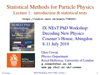
Statistical Tests and LimitsLecture 3 IN2P3 School of Statistics Autrans, France 17—21 May, 2010 Glen Cowan Physics Department Royal Holloway, University of London g.cowan@rhul.ac.uk www.pp.rhul.ac.uk/~cowan SOS 2010 / Statistical Tests and Limits -- lecture 3
Outline Lecture 1: General formalism Definition and properties of a statistical test Significance tests (and goodness-of-fit) , p-values Lecture 2: Setting limits Confidence intervals Bayesian Credible intervals Lecture 3: Further topics for tests and limits More on intervals/limits, CLs Systematics / nuisance parameters Bayesian model selection SOS 2010 / Statistical Tests and Limits -- lecture 3
Likelihood ratio limits (Feldman-Cousins) Define likelihood ratio for hypothesized parameter, e.g., for expected number of signal events s: Here is the ML estimator, note Critical region defined by low values of likelihood ratio. Resulting intervals can be one- or two-sided (depending on n). (Re)discovered for HEP by Feldman and Cousins, Phys. Rev. D 57 (1998) 3873. SOS 2010 / Statistical Tests and Limits -- lecture 3
Upper limit versus b Feldman-Cousins “Classical” Feldman & Cousins, PRD 57 (1998) 3873 If n = 0 observed, should upper limit depend on b? Classical: yes FC: yes, but less so SOS 2010 / Statistical Tests and Limits -- lecture 3
More on intervals from LR test (Feldman-Cousins) Caveat with coverage: suppose we find n >> b. Usually one then quotes a measurement: If, however, n isn’t large enough to claim discovery, one sets a limit on s. FC pointed out that if this decision is made based on n, then the actual coverage probability of the interval can be less than the stated confidence level (‘flip-flopping’). FC intervals remove this, providing a smooth transition from 1- to 2-sided intervals, depending on n. But, suppose FC gives e.g. 0.1 < s < 5 at 90% CL, p-value of s=0 still substantial. Part of upper-limit ‘wasted’? For this reason, one-sided intervals for limits still popular. SOS 2010 / Statistical Tests and Limits -- lecture 3
The Bayesian approach to limits In Bayesian statistics need to start with ‘prior pdf’ p(q), this reflects degree of belief about q before doing the experiment. Bayes’ theorem tells how our beliefs should be updated in light of the data x: Integrate posterior pdf p(q | x) to give interval with any desired probability content. For e.g. Poisson parameter 95% CL upper limit from SOS 2010 / Statistical Tests and Limits -- lecture 3
Bayesian prior for Poisson parameter Include knowledge that s≥0 by setting prior p(s) = 0 for s<0. Often try to reflect ‘prior ignorance’ with e.g. Not normalized but this is OK as long as L(s) dies off for large s. Not invariant under change of parameter — if we had used instead a flat prior for, say, the mass of the Higgs boson, this would imply a non-flat prior for the expected number of Higgs events. Doesn’t really reflect a reasonable degree of belief, but often used as a point of reference; or viewed as a recipe for producing an interval whose frequentist properties can be studied (coverage will depend on true s). SOS 2010 / Statistical Tests and Limits -- lecture 3
Bayesian interval with flat prior for s Solve numerically to find limit sup. For special case b = 0, Bayesian upper limit with flat prior numerically same as classical case (‘coincidence’). Otherwise Bayesian limit is everywhere greater than classical (‘conservative’). Never goes negative. Doesn’t depend on b if n = 0. SOS 2010 / Statistical Tests and Limits -- lecture 3
Priors from formal rules Because of difficulties in encoding a vague degree of belief in a prior, one often attempts to derive the prior from formal rules, e.g., to satisfy certain invariance principles or to provide maximum information gain for a certain set of measurements. Often called “objective priors” Form basis of Objective Bayesian Statistics The priors do not reflect a degree of belief (but might represent possible extreme cases). In a Subjective Bayesian analysis, using objective priors can be an important part of the sensitivity analysis. SOS 2010 / Statistical Tests and Limits -- lecture 3
Priors from formal rules (cont.) In Objective Bayesian analysis, can use the intervals in a frequentist way, i.e., regard Bayes’ theorem as a recipe to produce an interval with certain coverage properties. For a review see: Formal priors have not been widely used in HEP, but there is recent interest in this direction; see e.g. L. Demortier, S. Jain and H. Prosper, Reference priors for high energy physics, arxiv:1002.1111 (Feb 2010) SOS 2010 / Statistical Tests and Limits -- lecture 3
Jeffreys’ prior According to Jeffreys’rule, take prior according to where is the Fisher information matrix. One can show that this leads to inference that is invariant under a transformation of parameters. For a Gaussian mean, the Jeffreys’ prior is constant; for a Poisson mean m it is proportional to 1/√m. SOS 2010 / Statistical Tests and Limits -- lecture 3
Jeffreys’ prior for Poisson mean Suppose n ~ Poisson(m). To find the Jeffreys’ prior for m, So e.g. for m = s + b, this means the prior p(s) ~ 1/√(s + b), which depends on b. But this is not designed as a degree of belief about s. SOS 2010 / Statistical Tests and Limits -- lecture 3
Properties of upper limits Example: take b = 5.0, 1 - = 0.95 Upper limit sup vs. n Mean upper limit vs. s SOS 2010 / Statistical Tests and Limits -- lecture 3
Coverage probability of intervals Because of discreteness of Poisson data, probability for interval to include true value in general > confidence level (‘over-coverage’) SOS 2010 / Statistical Tests and Limits -- lecture 3
The “CLs” issue When the cross section for the signal process becomes small (e.g., large Higgs mass), the distribution of the test variable used in a search becomes the same under both the b and s+b hypotheses: f (q| b) f (q| s+b) In such a case we will reject the signal hypothesis with a probability approaching a = 1 – CL (i.e. 5%) assuming no signal. SOS 2010 / Statistical Tests and Limits -- lecture 3
The CLs solution The CLs solution (A. Read et al.) is to base the test not on the usual p-value (CLs+b), but rather to divide this by CLb (one minus the background of the b-only hypothesis, i.e., Define: f (q| b) f (q| s+b) q Reject signal hypothesis if: Reduces “effective” p-value when the two distributions become close (prevents exclusion if sensitivity is low). SOS 2010 / Statistical Tests and Limits -- lecture 3
CLs discussion In the CLs method the p-value is reduced according to the recipe Statistics community does not smile upon ratio of p-values; would prefer to regard parameter m as excluded if: (a) p-value of m < 0.05 (b) power of test of m with respect to background-only > some threshold (0.5?) Needs study. In any case should produce CLs result for purposes of comparison with other experiments. SOS 2010 / Statistical Tests and Limits -- lecture 3
Systematic errors and nuisance parameters Model prediction (including e.g. detector effects) never same as "true prediction" of the theory: model: y truth: x Model can be made to approximate better the truth by including more free parameters. systematic uncertainty ↔ nuisance parameters Statistical Methods in Particle Physics
Nuisance parameters and limits In general we don’t know the background b perfectly. Suppose we have a measurement of b, e.g., bmeas ~ N (b, b) So the data are really: n events and the value bmeas. In principle the exact confidence interval recipe can be generalized to multiple parameters, minimum coverage guaranteed. Difficult because of overcoverage; see e.g. talks by K. Cranmer at PHYSTAT03 and by G. Punzi at PHYSTAT05. G. Punzi, PHYSTAT05 SOS 2010 / Statistical Tests and Limits -- lecture 3
Nuisance parameters in limits (2) Connect systematic to nuisance parameters n. Then form e.g. Profile likelihood: Marginal likelihood: and use these to construct e.g. likelihood ratios for tests. Coverage not guaranteed for all values of the nuisance params. Results of both approaches above often similar, but some care is needed in writing down prior; this should truly reflect one’s degree of belief about the parameters. SOS 2010 / Statistical Tests and Limits -- lecture 3
Nuisance parameters and profile likelihood Suppose model has likelihood function Parameters of interest Nuisance parameters Define the profile likelihood ratio as Maximizes L for given value of m Maximizes L l(m) reflects level of agreement between data and m (0 ≤ l(m) ≤ 1) Equivalently use qm = -2 ln l(m) SOS 2010 / Statistical Tests and Limits -- lecture 3
p-value from profile likelihood ratio Large qm means worse agreement between data and m p-value = Prob(data with ≤ compatibility with m when compared to the data we got | m) chi-square cumulative distribution, degrees of freedom = dimension of m rapidly approaches chi-square pdf (Wilks’ theorem) Reject m if pm < g = 1 – CL (Approx.) confidence interval for m = set of m values not rejected. Coverage not exact for all n but very good if SOS 2010 / Statistical Tests and Limits -- lecture 3
Cousins-Highland method Regard b as ‘random’, characterized by pdf (b). Makes sense in Bayesian approach, but in frequentist model b is constant (although unknown). A measurement bmeas is random but this is not the mean number of background events, rather, b is. Compute anyway This would be the probability for n if Nature were to generate a new value of b upon repetition of the experiment with b(b). Now e.g. use this P(n;s) in the classical recipe for upper limit at CL = 1 - b: Result has hybrid Bayesian/frequentist character. SOS 2010 / Statistical Tests and Limits -- lecture 3
Marginal likelihood in LR tests Consider again signal s and background b, suppose we have uncertainty in b characterized by a prior pdf b(b). Define marginal likelihood as also called modified profile likelihood, in any case not a real likelihood. Now use this to construct likelihood ratio test and invert to obtain confidence intervals. Feldman-Cousins & Cousins-Highland (FHC2), see e.g. J. Conrad et al., Phys. Rev. D67 (2003) 012002 and Conrad/Tegenfeldt PHYSTAT05 talk. Calculators available (Conrad, Tegenfeldt, Barlow). SOS 2010 / Statistical Tests and Limits -- lecture 3
Comment on profile likelihood Suppose originally we measure x, likelihood is L(x|q). To cover a systematic, we enlarge model to include a nuisance parameter n, new model is L(x|q,n). To use profile likelihood, data must constrain the nuisance parameters, otherwise suffer loss of accuracy in parameters of interest. Can e.g. use a separate measurement to constrain n, e.g., with likelihood L(y|n). This becomes part of the full likelihood, i.e., SOS 2010 / Statistical Tests and Limits -- lecture 3
Comment on marginal likelihood When using a prior to reflect knowledge of n, often one treats this as coming from the measurement y, i.e., original prior, Then the marginal likelihood is So here L in the integrand does not include the information from the measurement y; this is included in the prior. SOS 2010 / Statistical Tests and Limits -- lecture 3
Bayesian limits with uncertainty on b Uncertainty on b goes into the prior, e.g., Put this into Bayes’ theorem, Marginalize over b, then use p(s|n) to find intervals for s with any desired probability content. Framework for treatment of nuisance parameters well defined; choice of prior can still be problematic, but often less so than finding a “non-informative” prior for a parameter of interest. SOS 2010 / Statistical Tests and Limits -- lecture 3
Bayesian model selection (‘discovery’) The probability of hypothesis H0 relative to an alternative H1 is often given by the posterior odds: no Higgs Higgs prior odds Bayes factor B01 The Bayes factor is regarded as measuring the weight of evidence of the data in support of H0 over H1. Interchangeably use B10 = 1/B01 SOS 2010 / Statistical Tests and Limits -- lecture 3
Assessing Bayes factors One can use the Bayes factor much like a p-value (or Z value). There is an “established” scale, analogous to our 5s rule: B10 Evidence against H0 -------------------------------------------- 1 to 3 Not worth more than a bare mention 3 to 20 Positive 20 to 150 Strong > 150 Very strong Kass and Raftery, Bayes Factors, J. Am Stat. Assoc 90 (1995) 773. Will this be adopted in HEP? SOS 2010 / Statistical Tests and Limits -- lecture 3
Rewriting the Bayes factor Suppose we have models Hi, i = 0, 1, ..., each with a likelihood and a prior pdf for its internal parameters so that the full prior is where is the overall prior probability for Hi. The Bayes factor comparing Hi and Hj can be written SOS 2010 / Statistical Tests and Limits -- lecture 3
Bayes factors independent of P(Hi) For Bij we need the posterior probabilities marginalized over all of the internal parameters of the models: Use Bayes theorem Ratio of marginal likelihoods So therefore the Bayes factor is The prior probabilities pi = P(Hi) cancel. SOS 2010 / Statistical Tests and Limits -- lecture 3
Numerical determination of Bayes factors Both numerator and denominator of Bij are of the form ‘marginal likelihood’ Various ways to compute these, e.g., using sampling of the posterior pdf (which we can do with MCMC). Harmonic Mean (and improvements) Importance sampling Parallel tempering (~thermodynamic integration) Nested sampling ... See e.g. SOS 2010 / Statistical Tests and Limits -- lecture 3
Harmonic mean estimator E.g., consider only one model and write Bayes theorem as: p(q) is normalized to unity so integrate both sides, posterior expectation Therefore sample q from the posterior via MCMC and estimate m with one over the average of 1/L (the harmonic mean of L). SOS 2010 / Statistical Tests and Limits -- lecture 3
Improvements to harmonic mean estimator The harmonic mean estimator is numerically very unstable; formally infinite variance (!). Gelfand & Dey propose variant: Rearrange Bayes thm; multiply both sides by arbitrary pdf f(q): Integrate over q : Improved convergence if tails of f(q) fall off faster than L(x|q)p(q) Note harmonic mean estimator is special case f(q) = p(q). . SOS 2010 / Statistical Tests and Limits -- lecture 3
Importance sampling Need pdf f(q) which we can evaluate at arbitrary q and also sample with MC. The marginal likelihood can be written Best convergence when f(q) approximates shape of L(x|q)p(q). Use for f(q) e.g. multivariate Gaussian with mean and covariance estimated from posterior (e.g. with MINUIT). SOS 2010 / Statistical Tests and Limits -- lecture 3
p-values versus Bayes factors Current convention: p-value of background-only < 2.9 × 10⁻⁷ (5s ) This should really depend also on other factors: Plausibility of signal Confidence in modeling of background Can also use Bayes factor Should hopefully point to same conclusion as p-value. If not, need to understand why! As yet not widely used in HEP, numerical issues not easy. SOS 2010 / Statistical Tests and Limits -- lecture 3
Summary Bayesian approach to setting limits is straightfoward; all information about the parameter is in the posterior probability, integrate this to get intervals with given probability. Difficult to find appropriate “non-informative” prior. Often use Bayesian approach as a recipe for producing interval, then study it in a frequentist way (e.g. coverage) The key to treating systematic uncertainties is to include in the model enough parameters so that it is correct (or very close). But too many parameters degrades information on parameters of interest Bayesian model selection Bayes factor = posterior odds if prior odds = 1. Only requires priors for internal parameters of models. Can be very difficult to compute numerically. SOS 2010 / Statistical Tests and Limits -- lecture 3