Download
1 / 28
310 likes | 616 Views
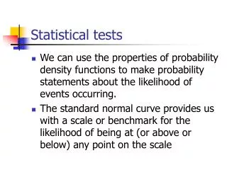
Statistical tests. We can use the properties of probability density functions to make probability statements about the likelihood of events occurring. The standard normal curve provides us with a scale or benchmark for the likelihood of being at (or above or below) any point on the scale.

E N D
Statistical tests • We can use the properties of probability density functions to make probability statements about the likelihood of events occurring. • The standard normal curve provides us with a scale or benchmark for the likelihood of being at (or above or below) any point on the scale
Standard normal values • Note for instance that if we look at the value 1.5 under the standard normal table, we find the value .4332. • This means that the probability of having a standard normal value greater than 1.5 is .5 - .4332 = .0668
In Applied Terms • If IQ has a mean of 100, and a standard deviation of 20, what is the probability that any given individuals IQ will be greater than or equal to 130. • Standardize the score of 130 • Look up 1.5 in the standard normal table
Two-tailed hypotheses • In general our hypothesis is: • Did the sample come from some particular population? • If the sample mean is too high or too low, we suspect that it did not. • Thus, we must check to see if the sample mean is either significantly higher, or significantly lower. • This is called a two-tailed test. • When in doubt, most tests are best done as two-tailed ones
The One Tailed Hypothesis • Sometimes we suspect, or hypothesize, direction • e.g. The average income for West Virginia will be significantly lower than the country as a whole. • HA: Xbar < • This is a one-tailed test • We ignore the tail in the direction not hypothesized
The Z-test • The z-test is based upon the standard normal distribution. • It uses the standard normal distribution in the same way. In this case we are making statements about the sample mean, instead of the actual data values
The Z-test – (cont.) • Note that the Z-test is based upon two parts. • The standard normal transformation • The standard deviation of the sampling distribution.
The Z-test – an example • Suppose that you took a sample of people off the street in Morgantown and found that their personal income is $19,362 • And you have information that the national average for personal income per capita is $26,412 in 1998. • Should you conclude that West Virginia is lower than the national average? • Is it significantly lower? • Could it simple be a “bad” sample” • How do you decide?
Example (cont.) • We will hypothesize that WV income is lower than the national average. • HA: WVInc < USInc (Alternate Hypothesis) • H0: WVInc = USInc (Null Hypothesis) • Since we know the national average ($26412) and standard deviation (4234), we can use the z-test to make decide if WV is indeed significantly lower than the nation
Example (cont.) • Using the z-test, we get
The Probability of a Type I error • We would like to not make mistakes. • We know we will. • With statistical inference, we have the ability to decide how often we find it acceptable to be wrong – by random chance. • Thus we set the probability of making a Type I error. • P(Type I error) = = ? • By convention =.05
The Critical Value of Z (cont) • Ok, now we know z… • We know that we can make probability statements about z, since it is from the standard normal distribution • We know that if z =1.96 then the area out in the tail past 1.96 is equal to .025 • This means that the likelihood of obtaining a value of z > 1.96 by random chance in any given sample is less than .025.
The Critical Values of Z to memorize • Two tailed hypothesis • Reject the null (H0) if z 1.96, or z -1.96 • One tailed hypothesis • If HA is Xbar > , then reject H0 if z 1.645 • If HA is Xbar < , then reject H0 if z -1.645
Z test example (cont.) • Suppose we decided to look at a different state, say Oregon with a mean of 24,766, and had a much smaller sample, say 16. • Using the z-test, we get • What would we conclude? • What if n=25? 100?
The t test • We frequently run into a problem with trying to do a z test. • While the population mean () may be frequently available, the population standard deviation () frequently is not. • Thus we use our best estimate of the population standard deviation – the sample standard deviation (s).
The t-test (cont.) • The t-test is a very similar formula. • Note the two differences • using s instead of • The resultant is a value that has a t-distribution instead of a standard normal one.
The t distribution • The t distribution
Two-sample t-test • Frequently we need to compare the means of two different samples. • Is one group higher/lower than some other group? • e.g. is the Income of blacks significantly lower than whites? • The two-sample t difference of means test is the typical way to address this question.
The Difference of means Test • The standard two-sample t-test is:
The equal Variance test • If the variances from the two samples are the same we may use a more powerful variation • Where
Contingency Tables • Often we have limited measurement of our data. • Contingency Tables are a means of looking at the impact of nominal and ordinal measures on each other. • They are called contingency tables because one variables value is contingent upon the other. • Also called cross-tabulation or crosstabs.
Contingency Tables • The procedure is quite simple and intuitively appealing • Construct a table with the independent variable across the top and the dependent variable on the side • This works fairly well for low numbers of categories (r,c < 6 or so)
Contingency Tables An example • Presidents are often suspected of using military force to enhance their popularity. • What do you suppose the data actually look like? • Any conjectures • Let’s categorize presidents as using force,or not, and as having popularity above and below 50% • Are their definition problems here? • Which is independent and which is dependent?
Measures of Independence • Are the variables actually contingent upon each other? • Is the use of force contingent upon the president’s level of popularity? • We would like to know if these variables are independent of each other, or does the use of force actually depend upon the level of approval that the president have at that time?
2 Test of Independence • The 2 Test of Independence gives us a test of statistical significance. • It is accomplished by comparing the actual observed values to those you would expect to see if the two variables are independent.
2 Test of Independence • Formula • Where