Statistical Tests
Statistical Tests . Statistical tests. Descriptive statistics : Description of observations Probability theory : Theoretical considerations ( no empirical data ) Statistical tests : Combination of descriptive statistics and probability theory

Statistical Tests
E N D
Presentation Transcript
Statistical tests • Descriptivestatistics: • Description ofobservations • Probabilitytheory: • Theoreticalconsiderations(noempiricaldata) • Statistical tests: • Combinationofdescriptivestatisticsandprobabilitytheory • Basedon observations (samples) conclusionsaredrawn • Caution: Conclusionsbased on statisticalinferenceareneverdeterministic • Conclusioncanalwaysbe „wrong“ • Minimal requirement: giveprobabilityforerror.
Statistical tests • General procedureofstatisticaltests: • Formulationofreasearchhypothesis (alternative hypothesis H1) andofformulationofthe null hypothesis H0 (hypothesisthatthereisnoeffect, typicallytheoppositeoftheresearchhypothesis). • Choice of an appropriatestatisticaltestandteststatistic • Choice ofrequiredlevelofsignficance. Oftenα =0.05 ischosen. This is an incrediblyweakcondition(personal opinion Tim Becker). • Computationofteststatisticfromdataandresultingdecision (rejectionoracceptanceof null hypothesis).
Statistical tests • Decidebetweentwo alternative hypothesesbased on information • Example: • Accusedatcourt • Information: witnesses, evidence, expert opinion, ... • Decision: guilty – not guilty • The judgehastwohypothesisforhisverdict: • H0: The accusedis not guilty (null hypothesis) • H1: The accusedisguilty (alternative hypothesis) • Whatcan happen?
1) Decision correct: Guilty gets acquittal 2) Decision correct: A guilty is convicted 3) Wrong decision: Innocent is convicted Example: Accusedatcourt 4) Wrong decision: Guilty gets acquittal Statistical tests H0: Accused is not guilty (Null hypothesis) H1: Accusedisguilty (Alternative hypothesis) Verdict Unknown truth H0 not guilty H1guilty H0 not guilty H1 guilty
Verdict Unknown truth H0 not guilty H1guilty H0 not guilty Type II error H1 guilty Type I error Situation 3: Type I error Situation 4: Type II error Statistical tests Errors of different kind and impact
Verdict Unknown truth H0 not guilty H1guilty H0 not guilty Type II error H1 guilty Type I error Statistical tests Terminology: Probability of type I error: Probability of type II error: Question: Which probability shall be made small? Answer: In principle both! Strategy: • Do not sentence innocents („minimize “) • Always decide not guilty • = 0 • Many guilties get acquittal • • Sentence all guilties („minimize “) • Always decide guilty • = 0 • Many innocents are sentenced •
Decision Unknown truth H0 H1 H0 Type II error () H1 Type I error () Statistical tests • Whicherror, or , ist worse? • can‘tbejudged in general,but depends on consideredhypotheses. Example 1: Case at court has to be minimized. „In dubio pro reo“ (innocent until proven guilty)
Decision Unknown truth old drug H0 New drug H1 H0 -old drug Type II error () H1 – new drug Type I error () Statistical tests Example 2: Is a new drug better than an established drug? H0: new drug is not betterH1: new, more expensive drug is better Type I error ():New drug will be given, although not better • Consequences: • Patient getunnecessary treatment • Treatment becomesmore expensive Type II error ():It is overlooked that the new drug is better • Consequences: • Patient does not getoptimaltreatment • Loss ofresearchcost
Decision Unknown truth No adverse re H0 Adverse re H1 H0 -no adverse reaction Type II error () H1 – adverse reaction Type I error () Statistical tests Example 3: Does the drug lead to severe adverse reaction? H0: Drug does not leadtoadversereactionH1: Drug doesleadtoadversereaction Type I error ():Adverse reaction is assumed, although not present Type II error ():Severe adverse reaction is not recognized Consequence: Type II error () has to be minimized
Statistical tests Formulationofhypotheses
Blood pressure is lowered Great drug ??? Statistical tests Example: Drug to lower blood pressure H0: Drug does not workH1: Drug works 1) How to measure the effect? Definetargetvalue X X: systolic blood pressure in mmHg 2) Investigation Patient: Measurement before drug intake: 190 mmHg Measurement after drug intake: 185 mmHg H1 correct??? Difference may be a chance effect ! Patient: Measurement before drug intake :190 mmHg Measurement after drug intake :140 mmHg Difference may be an individual effect Sample / independentrepetition
Patient xi before xi after difference di 1 190 185 5 2 185 175 10 3 180 185 -5 4 180 180 0 5 190 170 20 n 190 175 15 Statistical tests Decisiondepends on meanof „reduction in bloodpressure“ • Conclusion on reductionofbloodpressureshallbemade • Conclusion on expectationμd oftargetvalue X shallbemade
Statistical tests Conclusion on reductionofbloodpressureshallbemade Hypotheseswithrespecttotargetvalue X must beformulated in termsoftheexpectation Twotypesofhypotheseshavetobedistinguished: One-sidedhypotheses: X: targetvalue: reductionofbloodpressure in mmHg H0: Drug does not work: μd = 0 (μd ≤ 0) H1: Drug works: μd > 0 Tow-sidedhypotheses: X: targetvalue: reductionofbloodpressure in mmHg H0: Drug does not work: μd = 0 H1: Drug works: μd 0
Statistical tests One-sidedtest
Sample Patient before after difference 1 190 185 5 2 180 185 -5 50 190 175 15 n=50 d 20 0 All we have is one sample with Statistical tests X: „reduction of blood pressure“ [mmHg] H0: μd = 0 H1: μd > 0 Make decision
H0 H1 20 0 Statistical tests Decision: H0 is true H1 is true Decision „changes“ at a limitthatneedspre-specification.
Sample Patient before after difference 1 190 185 5 2 180 185 -5 5% n 190 175 15 0 Itisthe 95% - quantileof Statistical tests H0: μd = 0H1: μd> 0 One-sided question α = 5 % Limit has to be pre-specified! Limit isimplicitlygivenby. Whatisthelimitforα = 5 %?
Statistical tests Two-sidedtest
Statistical tests Test statistic – t test
Sample Patient before after difference 1 190 185 5 2 180 185 -5 n 190 175 15 t 0 • Mean of the differences Test statistic t Statistical tests HypothesesH0: μd = 0H1: μd0 = 5 % What shall decision depend on? • Standard deviation s • Sample size n
sample Patient before after difference 1 190 185 5 2 180 185 -5 n 190 175 15 0 t Statistical tests • T-test forpairedsamples target: reduction in bloodpressure d Hypotheses H0: μd= 0 vs. H1: μd 0(two-sidedtest) = 5 % Test statistict (In R: t.test() ): In case(!) diisnormallydistributed: • tist - distributedwith (n-1) degreesoffreedom „Student‘s t-Test“
Statistical tests Quantiles tf;0.95and tf;0.975 ofthetf– distribution
sample target: reduction in blood pressure d H0: μd= 0 vs. H1: μd 0(two-sided) = 5 % Patient before after difference 1 190 185 5 2 180 185 -5 15 190 175 15 2,5% 2,5% 0 -2,145 2,145 6,21 t n=15 f=n-1=14 p= f= 0,950 0,975 13 14 15 20 1.771 1.761 1.753 1.725 2.160 2.145 2.131 2.086 t = 6,21 > 2,145 = t14; 0.975 Statistical tests Decision Compare t = 6,21 with Quantile Decision: H0 is discardedH1 is accepted=5 %
Statistical tests • Rejection criteria: • One-sidedhypothesis: • : vs. : : rejectioninterval : • : vs. : : rejectioninterval: • canberejected a • Tow-sidedhypothesis: • :canberejectedatif or , i.e. if • : can berejectedatif is not located in the()100%-confidenceintervall:
Therapy A Hypotheses: H0: = 0H1: 0 Therapy B Patient Patient blood pr blood pr 1 1 150 140 2 2 135 125 3 3 140 130 nA nB 132 145 μA μB Statistical tests • T-test forun-pairedsamples Example: Blood pressure after 3 months, fortwo different therapies Question:Isthere a differencebetweentherapy A andtherapy B? Hypotheses: H0: μA = μBH1: μAμB Wearelookingfor a judgementaboutthedifferenceoftheunknownmeanvaluesμAandμB
Therapy A Therapy B Patient Patient Blood pr Blood pr 1 1 150 140 2 2 125 135 Test statistic: 3 3 140 130 nB nA 145 132 test statistic t is t – distributed with (nA + nB -2) degrees of freedom Statistical tests Hypotheses: H0: μA = μBH1: μAμB (two-sided) = 5 % Parameters for a test statistic t? Assumption: XA N(μA; σA2) XB N(μB; σB2) mit σA2= σB2
Therapy A -2,021 2,021 Therapy B Patient Patient Blutdruck Blutdruck 1 1 150 140 2 2 135 125 3 3 140 130 2,5% 2,5% nA nB 132 145 2,21 0 t Statistical tests Hypotheses: H0: μA = μBH1: μAμB (two-sided) = 5 % XA N(μA; σA2)XB N(μB; σB2) σA2= σB2 Decision: Reject H0Accept H1=5 % Compare t = 2,21 with the quantile of the t-distribution (nA=20, nB=22 f=nA+nB-2=40) t = 2,21 > 2,021 = t40; 0.975
Statistical tests • Rejectioncirteria: • One-sidedhypothesis: • : vs. : : canberejectedifatif • :vs. : : can berejectedifatif • Tow-sided hypothesis: • : bzw. :can berejectedifatif 0is not locatcted in the()100%-confidenceinterval:
Test statistic: Statistical tests • T-test forun-pairedsampleswith different variancesσA2σB2 Hypothesesunchanged:H0: μA= μBvs. H1: μAμB (two-sided)= 5 % Parameters for Welch t test? • If, then
teststatistic tist – distributedwith degreesoffreedom Statistical tests • Rejectioncriterion: • can be rejected at if Assumption: XA N(μA; σA2) XB N(μB; σB2) mit σA2σB2
Statistical tests -test
Expected under H0 Observed Post-op intricacies OP-Type Post-op intricacies OP-Type A B A B yes 55 yes 12 43 55 no 29 no 5 24 29 17 67 84 17 67 84 Statistical tests • Testingcategorial variables Here, „expected“ means that we assume that the op-type has no impact on whether post-op intircacies will occur or not
Expected Observed Post-op intricacies OP-Type Post-op intircacies OP-Type A B A B yes 55 yes 12 43 55 no 29 no 5 24 29 17 67 84 17 67 84 Test statistic (In R: chisq.test() ): Statistical tests Test statistic is 2-distributed with f = 1 degree of freedom
Expected Observed Post-op problems OP-Type Post-op problems OP-Type A B A B yes 55 yes 12 43 55 no 29 no 5 24 29 17 67 84 17 67 84 Test statistic: Statistical tests Hypotheses: H0: OP-Type and postoperative intricaciesareindependent H1: ..are not independent = 5 % Two-sidedtest. Compare 2 to quantile of 2 -distribution (degrees of freedom f=1) 2 = 0,26 < 3,814 = 2 1;0.95 Decision: H0 can not be rejected
Test statisitc: Statistical tests • Simplificationfor 2-by-2 tables Quantile2 1;0.95 = 3,814 Degreesoffreedom: f = 1 Decision: 2 3,814: H0can not berejected. 2 > 3,814: H0canberejected.
Statistical tests • General (k x m)-contingencytables: • : Variable 1 and variable 2 areindependent vs. : variable 1 andvariable 2 are not independent • observedfrequencies • expectedfrequencies
Statistical tests • Test statistic: • is under asymptotically ²-distributed with (k-1)(m-1) degressoffreedom. • Rejectioncriterion: • canberejectedatif², where k isthenumberofrowsand m isthenumberofcolumns. • The approximationoftheteststatisticwiththe² -distribution isacceptableiffor 80% ofthecellstheexpected(!) numberofcellcountsis >=5. OtherwiseuseFisher‘sexacttest(cf. Follwingpresentations).
Statistical tests Relative Riskand Odds Ratio
Statistical tests • Relative Risk: • A measureforriskdifferencebetweentwogroups. • Itisthethefactorbywhichtheriskisincreased • X=1: individual isexposedtoriskfactor • X=0: individual is not exposed • K=1: individual hasdisease • K=0: individual does not havethedisease • Conditionalprobabilitytobeill, underexposure : P(K=1|X=1) • Conditionalprobabilitytobeillwithoutexposure : P(K=1|X=0)
Statistical tests 2x2 tableofprobabilities P(K=0|X=0)= P(K=0|X=1)= P(K=1|X=0)= P(K=1|X=1)= • Relative risk
Statistical tests • Odds ratio • odds(A)ratioofprobabilityandprobabilityofoppositeevent • Whentheprobabilites, theprobabilitesareestiamtedandthe OR iscomputedasfollows: 2 x 2 tableofobservedfrequencies
Statistical tests Example: Retrospectivestudytodetectif Tonsillektomie increasesriskfor Morbus Hodgkin => Propabilitytogetthedisease in increasedunderexposure (Tonsillektomie)
Statistical tests • Correspondingstatisticaltest • canberejected, if 1 is not located in the()100%-confidenceintervallof OR:
Statistical tests • Beispiel: Retrospektive Studie, ob Tonsillektomie das Risiko für Morbus Hodgkin erhöht • , • ()100%-Konfidenzintervall für OR: • kann zum Niveau verworfen werden, da 1 nicht im ()100%-Konfidenzintervall liegt.