Addressing
Addressing. By Tamanna Sait & Aneesha Deo. Introduction. IP Network Addressing Internet Scaling Problems Classful IP Addressing Subnet Addressing Variable Length Subnet Masks (VLSM) Classless Inter-Domain Routing (CIDR) Routing Protocols in Internet Routing Information Protocol (RIP)


Addressing
E N D
Presentation Transcript
Addressing By Tamanna Sait & Aneesha Deo
Introduction • IP Network Addressing • Internet Scaling Problems • Classful IP Addressing • Subnet Addressing • Variable Length Subnet Masks (VLSM) • Classless Inter-Domain Routing (CIDR) • Routing Protocols in Internet • Routing Information Protocol (RIP) • Open Shortest Path First (OSPF) • Border Gateway Protocol (BGP)
IP Network Addressing • Today, the Internet has entered the public consciousness as the world’s largest public data network, doubling in size every nine months • There is a direct relationship between the value of the Internet and the number of sites connected to the internet • The internet has experienced two major scaling issues as it has struggled to provide continuous and uninterrupted growth
Internet Scaling Problems • The first problem is concerned with the eventual depletion of the IP address space • The current version of IP, IP version 4 (IPv4), defines a 32-bit address which means that there are only 232 (4,294,967,296) IPv4 addresses available • IP address space has not been efficiently allocated • Traditional model of classful addressing does not allow the address space to be used to its maximum potential.
Internet Scaling Problems • The second problem is caused by the rapid growth in the size of the Internet routing tables • Internet backbone routers are required to maintain complete routing information for the Internet • Over recent years, routing tables have experienced exponential growth • Unfortunately, the routing problem cannot be solved by simply installing more router memory and increasing the size of routing tables
Internet Scaling Problems • Other factors related to the capacity problem include: • growing demand for CPU horsepower to compute routing table/topology tables • increasing nature of WWW connections and their effect on router forwarding caches • volume of information to be managed by people and machines
Internet Scaling Problems • The long term solution to these problems can be found in the widespread deployment of IP Next Generation or IPv6 • Classless Inter domain Routing (CIDR) is a solution to efficiently utilize the existing address space
Classful IP Addressing • When IP was first standardized in Sep 1981, each system attached to the IP based Internet had to be assigned a unique 32-bit address • The 32-bit IP addressing scheme involves a two level addressing hierarchy Network Number/Prefix Host Number
Classful IP Addressing • Network number is also referred to as the network prefix • All hosts on a given network share the same network prefix but have a unique host number • Two hosts on different networks must have different network prefixes but may have the same host number
Classful IP Addressing • IP address space is divided into 3 different address classes – Class A, Class B and Class C • Each class fixes the boundary between the network-prefix and the host number at a different point in the 32-bit address
Classful IP Addressing • Class A network has an 8-bit network prefix with the highest order bit set to 0 and a seven-bit network number, followed by a 24-bit host-number • A maximum of 126 (27 – 2)/8 networks can be defined Class A 0 1 7 8 31 0
Classful IP Addressing • Class B network has a 16-bit network prefix with the 2 highest order bit set to 1-0 and a 14-bit network number, followed by a 16-bit host-number • A maximum of 16,384 (214)/16 networks can be defined with up to 65,534 (216 – 2) hosts/network Class B 0 2 15 16 31 10
Classful IP Addressing • Class C network has a 24-bit network prefix with the 3 highest order bit set to 1-1-0 and a 21-bit network number, followed by a 8-bit host-number • A maximum of 2,097,152 (221)/24 networks can be defined with up to 254 (28 – 2) hosts/network Class C 0 3 23 24 31 110
Classful IP Addressing • Class D addresses have their leading 4-bits set to 1-1-1-0 and are used to support Multicasting • For example: • 224.0.0.1 All systems on LAN • 224.0.0.2 All routers on LAN • 224.0.0.5 All OSPF routers on LAN Class D 0 4 31 Multicast Address 1110
Classful IP Addressing • Class E addresses have their leading 5-bits set to 1-1-1-1-0 • Reserved for experimental/future purpose Class E 0 5 31 Reserved for Future use 11110
Subnetting • Subnet addressing is used by system administrators in order to further subdivide an Internet address within an organization • Instead of the classful two-level hierarchy, subnetting supports a three-level hierarchy Network-Prefix Host-Number Network-Prefix Subnet-Number Host-Number
Subnetting • Subnetting attacked the expanding routing problem by ensuring that the subnet structure of a network is never visible outside of the organization’s private network • The route from the Internet to any subnet of a given IP address is the same, no matter which subnet the destination host is on • All subnets of a given network number use the same network-prefix but different subnet numbers
Subnetting Extended-Network-Prefix • Routers within the subnetted environment use the extended-network-prefix to route traffic between the individual subnets • The extended-network-prefix is composed of the classful network-prefix and the subnet-number • The extended-network-prefix has traditionally been identified by the subnet mask
Subnetting – Example US Europe Subnet B network #: 00001011.100 11.32.0.0 R R R R Subnet A R 11.0.0.0 network #: 00001011.000 Subnet C 11.64.0.0
Subnetting – Example • Given: • US has 3 locations, each with a router • Europe has 2 locations with routers • Class A IP Address of 11.0.0.0 has been obtained • Need: • To create unique network numbers for each side of the routed network
Subnetting – Example • We need to decide which bits of the host address to use as a part of the network number • Keep all network bits on the left and the host numbers on the right hand side of the IP address • We use the highest three bits of the host address area for the subnet mask • The bits of our address are divided into Network number: nnnnnnnn.ssshhhhh.hhhhhhhh.hhhhhhhh
Subnetting – Example • The first bit of the subnet will equal 0 if the packet is to be routed to the US, and 1 if it is to be routed to Europe • The remaining two bits will be used to differentiate the routers within the continent • For example, routers in the US will have the subnet mask values of • 000 Subnet A • 001 Subnet B • 010 Subnet C
Subnetting – Example • The network numbers of the subnets in the US are 00001011.00000000.00000000.00000000 11.0.0.0 00001011.00100000.00000000.00000000 11.32.0.0 00001011.01000000.00000000.00000000 11.64.0.0 • Because the subnet bits have been divided logically based on their routes, it will be easier to determine which subnet a packet is destined for
Subnetting – Example • For this example, given Class A address of 11.0.0.0 and a subnet mask of 255.255.0.0 and one of the workstations in the US had an IP address of 11.1.1.69, the network portion is 11.1.1.69 00001011.00000001.00000001.01000101 & 255.255.0.0 11111111.11111111.00000000.00000000 11.1.0.0 00001011.00000001.00000000.00000000
Subnetting – Example • To find the destination address for a directed broadcast for net 11.1.0.0, take the ~ of the subnet mask then bitwise OR it with the IP address 11.1.1.69 00001011.00000001.00000001.01000101 | 0.0.255.255 00000000.00000000.11111111.11111111 11.1.255.255 00001011.00000001.11111111.11111111
Variable Length Subnet Masks (VLSM) • When an IP network is assigned more than one subnet mask, it is considered a network with “variable length subnet masks” since the extended-network-prefixes have different lengths • VLSM allows the recursive division of an organization’s address space so that it can be reassembled and aggregated to reduce the amount of routing information at the top level
Classless Inter-Domain Routing (CIDR) Disadvantages of Classful IP Routing • The near-term exhaustion of the Class B network address space • The rapid growth in the size of the global Internet’s routing tables • The eventual exhaustion of the 32-bit IPv4 address space
Classless Inter-Domain Routing (CIDR) CIDR supports two important features that benefit global Internet routing system • Eliminates the traditional concept of Class A, Class B and Class C network addresses, which enables efficient allocation of IPv4 address space • Supports route aggregation where a single routing table entry can represent the address space of thousands of traditional classful routes
Classless Inter-Domain Routing (CIDR) Efficient allocation of the IPv4 address space • Replaces the traditional concept of Classful addresses with the generalized concept of a “network-prefix” • Network-prefix determines the dividing point between the network and the host number • Supports the deployment of arbitrarily sized networks rather than the standard 8-bit, 16-bit or 24-bit network numbers associated with Classful addressing
Classless Inter-Domain Routing (CIDR) • Each piece of routing information is advertised with a bit mask or prefix length which specifies the number of leftmost contiguous bits in the network portion of each routing table entry • All prefixes with same prefix length represent same amount of address space • For example, a/20 represents a network with a 20 bit prefix length and 12 bit host number and can support up to 212 (4096) host addresses
Classless Inter-Domain Routing (CIDR) Minimization of Routing table entries • A single routing table entry can specify how to route traffic to many individual network addresses. • The world is partitioned into 4 zones and each one is given a portion of Class C address space. Addresses 194.0.0.0 – 195.255.255.255 -> Europe Addresses 198.0.0.0 – 199.255.255.255 -> N. America Addresses 200.0.0.0 – 201.255.255.255 -> C. & S. America Addresses 202.0.0.0 – 203.255.255.255 -> Asia & Pacific
Classless Inter-Domain Routing (CIDR) • 32 million addresses to allocate, with another 320 million class C addresses from 204.0.0.0 through 223.255.255.255 held in reserve for the future use • The advantage of this allocation is that now any router outside of Europe that gets a packet addressed to 194.xx.yy.zz or 195.xx.yy.zz can send it to its standard European Gateway, thus reducing the routing table entry to 1 entry
Classless Inter-Domain Routing (CIDR) • Each routing table entry consists of a base address and a 32-bit mask • When a packet comes in, its destination address is first extracted • The routing table is scanned, masking the destination address and comparing to the table entry looking for a match
Classless Inter-Domain Routing (CIDR) Example Routing Table Entry
CIDR Table Entry • Extract the destination IP address. • Boolean AND the IP address with the subnet mask for each entry in the routing table. • The answer you get after ANDing is checked with the base address entry corresponding to the subnet kask entry with which the destination entry was Boolean ANDed. • If a match is obtained the packet is forwarded to the router with the corresponding base address
Routing Algorithms • Routing is the process of forwarding messages through switching networks • Routing information is stored in Routing Tables • These tables contain the path information as well as cost • Routing can be decided in two ways • Static Route Selection – routing info provided manually • Dynamic Route Selection – Distance Vector and Link State Routing
Routing In The Internet • The Internet can be viewed as a collection of sub networks or autonomous systems(AS). • Routing in the Internet involves routing within and between autonomous systems(AS). • Protocol used for routing within the autonomous system is “Interior Gateway Protocol” which includes: • Routing Information Protocol(RIP) • Open Shortest Path First Protocol(OSPF) • Protocol used for routing between autonomous systems is “Exterior Gateway Protocol” or “Border Gateway protocol”(BGP)
Routing Information Protocol (RIP) • RIP is a distance-vector protocol • Using RIP, a gateway host (with a router) sends its entire routing table to its closest neighbor host every 30 seconds • The neighbor host in turn will pass the information on to its next neighbor and so on • RIP uses a hop count as a way to determine network distance • RIP messages are carried in UDP datagrams, maximum datagram size 512 octets
Routing Information Protocol (RIP) Version 0 Command (1-6) 0 Address Family 32-bit IP address 0 0 metric 24 more routes
Routing Information Protocol (RIP) • Benefits • The only interior gateway protocol that can be counted on to really run everywhere • Configuring a RIP system requires little effort • RIP uses an algorithm that does not impose serious computation or storage requirements on hosts and routers
Routing Information Protocol (RIP) • Limitations • Does not solve every possible routing problem • The protocol is limited to networks whose longest path involves 15 hops • The entire routing table is sent every 30 sec, which increases traffic • The protocol suffers from “counting to infinity” problem • This protocol uses fixed “metrics” to compare alternative routes. It is not appropriate for situations where routes need to be chosen based on real-time parameters such as measured delay, reliability or load
Open Shortest Path First (OSPF) • OSPF supports 3 kinds of connections and networks: • Point-to-point links between exactly two routers • Multiaccess networks with broadcasting • Multicasting networks without broadcasting • OSPF works by abstracting a collection of actual networks,routers and lines into a directed graph in which each arc is assigned a cost. • Shortest path is computed based on weights on the arcs
Example Network and Graph for OSPF WAN 1 B A C D E F G W1 LAN 1 LAN 2 B C A 4 E 10 F 44 10 3 D 4 2 2 2 G 3 L2 L1
Open Shortest Path First (OSPF) • OSPF allows ASes to be divided into numbered areas, which is a generalization of a subnet • Outside an area, its topology is not visible • Every AS has a backbone area called area 0 and all other areas are connected to this backbone • All inter-area packet routing takes place via backbone area or area 0 • Each router that is connected to two or more areas is part of the backbone
Open Shortest Path First (OSPF) BGP protocol connects the ASes Backbone AS 1 AS 2 Backbone router Area Internal router Area border router AS 4 AS 3 AS boundary router
Open Shortest Path First (OSPF) • Using flooding, each router informs all other routers in its area of its neighbors and its cost • This information allows each router to construct a graph for its area and compute its shortest path • The backbone routers, in addition to this, accept information from the Area Border Routers to compute the best route to every other router • This information is propagated back to Area Border Routers and advertised within their areas
Open Shortest Path First (OSPF) • Limitations • It is complex because it divides the AS into a number of areas • For the traffic to travel between two areas, it must be first routed to the backbone (area 0). This may cause non-optimal routes • Although link-state protocols are not difficult to understand, OSPF muddles the picture with plenty of options and features
Border Gateway Protocol (BGP) • BGP is an exterior gateway protocol • BGP has been designed to allow many kinds of routing policies to be enforced in the interAS traffic • These policies are manually configured and are not a part of the protocol • Typical policies involve political, security or economic considerations. For example • Traffic starting or ending at IBM should not transit Microsoft • No transit traffic through certain AS systems
Border Gateway Protocol (BGP) • From the point of view of a BGP router, the world consists of other BGP routers and the lines connecting them • Based on transit traffic, networks are grouped into one of the three categories • Stub networks: Have only one connection to the BGP graph and cannot be used for transit traffic • Multi-connected: Could be used for transit traffic unless they refuse • Transit Networks (Backbones): These networks are willing to handle third party packets with some restrictions
Border Gateway Protocol (BGP) • BGP is fundamentally a distance vector protocol with some modifications • Instead of maintaining a cost to each destination, each BGP router keeps a track of the exact path used • BGP peers initially exchange their full routing tables • Thereafter, they exchange routing updates only