Addressing
Addressing. A large portion of the bits in a program are used to specify where the operands come from rather than what operations are being performed on them. An ADD instruction requires the specification of three operands: two sources and a destination.

Addressing
E N D
Presentation Transcript
Addressing • A large portion of the bits in a program are used to specify where the operands come from rather than what operations are being performed on them. • An ADD instruction requires the specification of three operands: two sources and a destination. • If memory addresses are 32 bits, the instruction takes three 32-bit addresses in addition to the opcode. • Two general methods are used to reduce the size of the specification
Addressing • If an operand is to be used several times, it can be moved to a register. • To do this, we must perform a LOAD (which includes the full memory address). • A second method is to specify one or more addresses implicitly. • Use a two-address instruction, for example. • The Pentium II uses two-address instructions while the UltraSPARC II uses three-address instructions. • If we have instructions which can work with only one register, we can have one-address instructions. • Finally, using a stack we can have zero-address instructions (the JVM IADD, for example).
Addressing Modes • There are many different ways we can specify addresses. These are called addressing modes. • The simplest way for an instruction to specify an operand is to include the operand rather than an address or some other information describing where the operand is. This is called immediate addressing and the operand is called an immediate operand. • This only works with constants. • The number of values is limited by the size of the field.
Direct Addressing • A method for specifying an operand in memory is just to give its full address. This is called direct addressing. • The instruction will always access exactly the same memory location. • Thus direct addressing can only be used to access global variables whose address is known at compile time. • Many programs have global variables so this method is widely used.
Register Addressing • Register addressing is conceptually the same as direct addressing but specifies a register rather than a memory location. • Because registers are so important this addressing mode is the most common one on most computers. • Many compilers determine the most frequently used variables and place them in registers. • This addressing mode is known as register mode. • In load/store architectures such as the UltraSPARC II, nearly all instructions use this addressing mode exclusively.
Register Indirect Addressing • In this mode, the operand being specified comes from memory or goes to memory, but its address is not hardwired into the instruction, as in direct addressing. • Instead the address is contained in a register. • When an address is used in this manner it is called a pointer. • Register indirect addressing can reference memory without having a full memory address in the instruction.
Register Indirect Addressing • The previous program used several addressing modes. • The first three instructions use register mode for the first operand, and immediate mode for the second operand (a constant indicated by the # sign). • The body of the loop itself does not contain any memory addresses. It uses register and register indirect mode in the fourth instruction. • The BLT might use a memory address, but mode likely it specifies the address to branch to with an 8-bit offset relative to the BLT instruction itself.
Indexed Addressing • It is frequently useful to be able to reference memory words at a known offset from a register. (Remember in IJVM we referenced local variables by giving their offset from LV). • Addressing memory by giving a register (explicit or implicit) plus a constant offset is called indexed addressing. • We can also give a memory pointer in the instruction and a small offset in the register
Based Indexed Addressing • Some machines have an addressing mode in which the memory address is computed by adding up to registers plus an (optional) offset. • Sometimes this mode is called based-indexed addressing. • One of the registers is the base and the other is the index. • We could have used this mode in the previous program to write: LOOP: MOV R4, (R2+R5) AND R4, (R2+R6)
Stack Addressing • We have noted that it is desirable to make machine instructions as short as possible. • The ultimate limit in reducing address lengths is having no addresses at all. • As we have seen, zero-address instructions, such as IADD are possible in conjunction with a stack. • It is traditional in mathematics to put the operator between the operands (x + y), rather than after the operands (x y +). • Between the operands is called infix notation. • After the operands is called postfix or reversePolish notation.
Reverse Polish Notation • Reverse Polish notation has a number of advantages over infix for expressing algebraic formulas. • Any formula can be expressed without parentheses. • It is convenient for evaluating expressions on computers with stacks. • Infix operators have precedence, which is arbitrary and undesirable. • There are several algorithms for converting infix formulas into Polish notation. This one is by Dijkstra.
Reverse Polish Notation • Assume that a formula is composed of the following symbols: variable, the dyadic (two-operand) operators + - * /, and left and right parentheses. A special symbol marks the ends of a formula. • The following slide shows a railroad track from New York to California with a spur that goes to Texas. Each symbol in the formula is represented by a railroad car. The train moves westward. • Cars containing variables always go to California. The special symbol always go to Texas.
Reverse Polish Notation • The other symbols must inquire about the contents of the nearest car on the Texas line before entering the switch. The possibilities are: 1. The car at the switch heads toward Texas. 2. The most recent car on the Texas line turns and goes to California. 3. Both the car at the switch and the most recent car on the Texas line are hijacked and disappear (i.e. both are deleted). 4. Stop. The symbols now on the California line represent the RPN formula read from left to right. 5. Stop. The original formula contained an error.
Reverse Polish Notation • RPN is the ideal notation for evaluating formulas on a computer with a stack. • The formula consists of n symbols, each one either an operand or an operator. • Scan the RPN string from left to right. When an operand is encountered, push it onto the stack. When an operator is encountered, execute the corresponding instruction. • The following figure shows the evaluation of (8 + 2 X 5) / (1 + 3 X 2 - 4) in JVM. The corresponding RPN formula is 8 2 5 X + 1 3 2 X + 4 - /
Addressing Modes for Branch Instructions • Branch instructions (and procedure calls) also need addressing modes for specifying the target address. • The modes we have examined so far also work for branches for the most part. • However, other addressing modes also make sense. • Register indirect addressing allows the program to compute the target address, put it in a register, and then go there. The target address is computed at run time.
Addressing Modes for Branch Instructions • Another reasonable mode is indexed mode, which offsets a known distance from a register. It has the same properties as register indirect mode. • Another option is PC-relative addressing. In this mode, the (signed) offset in the instruction itself is added to the program counter to get the target address. • In fact, this is simply indexed mode, using PC as the register.
Orthogonality of Opcodes and Addressing Modes • Instructions and addressing should have a regular structure, with a minimum number of instruction formats. • Such a structure makes it easier for a compiler to produce good code. • All opcodes should permit all addressing modes, where that makes sense. • All registers should be available for all register modes. • The following slide shows an example of a clean design for a three operand machine.
Orthogonality of Opcodes and Addressing Modes • Up to 256 opcodes are supported. • In format 1, each instruction has a two source registers and a destination register. • All arithmetic and logical instructions use this format. • The unused 8-bit field at the end can used for further instruction differentiation. • If bit 23 is set, format 2 is used and the second operand is no longer a register but a 13-bit signed immediate constant. LOAD and STORE can also use this format in indexed mode.
Orthogonality of Opcodes and Addressing Modes • A small number of additional instructions are needed, such as conditional branches, but they could easily fit in format 3. • For example, one opcode could be assigned to each (conditional) branch), procedure call, etc., leaving 24 bits for a PC relative offset. Assuming that this offset counted in words, the range would be 32 MB. • Also a few opcodes could be reserved for LOADs and STOREs that need the long offsets of format 3. • A design for a two-address machine is shown on the following slide.
Instruction Types • There are several groups of instruction types: • Data Movement Instructions • Dyadic Operations • Monadic Operations • Comparison and Conditional Branches • Procedure Call Instructions • Loop Control • Input/Output
Instruction Types • Data Movement Instructions • Might better be called data duplication instructions. • LOAD - memory to register • STORE - register to memory • MOVE - register to register
Instruction Types • Dyadic Operations • Addition/Subtraction • Multiplication/Division • Boolean Operations: AND, OR, XOR, NOR, NAND. • AND can be used to extract bits from a word by ANDing together the word with a constant mask. • The result is shifted to obtain the correct bits.
Instruction Types • Monadic Operations • SHIFT and ROTATE • Can be used to implement multiplication and division by powers of 2. • INCREMENT and DECREMENT • NEG
Instruction Types • Comparison and Conditional Branches • We may need to test a condition before branching to a statement beginning with a LABEL. • Some machines have condition bits that are used to indicate specific conditions. • Carry bit, for example. • Branch if a word is zero is an important instruction. • Can also compare two words - a comparison bit is set.
Instruction Types • Loop control • The need to execute a group of instructions a fixed number of times occurs frequently and thus some machines have instructions to facilitate this. • All the schemes involve a counter that is increased or decreased by some constant once each time though the loop. • The counter is also tested once each time through the loop. • If a certain condition holds, the loop is terminated.
Instruction Types • Input/Output • Three different I/O schemes are in current use in PCs: • Programmed I/O with busy waiting • Interrupt-driven I/O • DMA I/O • In programmed I/O, the CPU usually have a single input instruction and a single output instruction. • A single character is transferred between a fixed register and the selected I/O device.
Instruction Types • The primary disadvantage of programmed I/O is that the CPU wastes time in a tight loop. • This is called busy waiting. • This is OK in embedded processors, but not in a multitasking machine. • We can avoid this problem by starting the I/O and telling the I/O device to generate an interrupt when it is done. • In Direct Memory Access (DMA), a chip connected directly to the bus relieves the CPU of processing the interrupts.
Traps • A trap is a kind of automatic procedure call initiated by some condition caused by the program. • Common conditions include • floating-point overflow/underflow • integer overflow/underflow • protection violation • divide by zero • undefined opcode • A trap handler routine is invoked.
Interrupts • An interrupt is a change in the flow of control caused not by the running program, but by something else, usually related to I/O. • The essential difference between traps and interrupts is that traps are synchronous with the program and interrupts are asynchronous. • Rerunning a program will always generate the same traps but not the same interrupts. • An interrupt routine should be transparent.
The Intel IA-64 • The IA-64 is the next generation of processors developed by Intel (along with HP). • It is a completely new architecture. • It is a full 64-bit architecture. • Also known as Merced. • Initially to be used for high-end servers.
The Intel IA-64 • Problems with the IA-32 architecture: • Variable-length instructions and formats • Two-address memory-oriented ISA • Small and irregular register set • Register renaming, out-of-order execution, in-order retiring require very complex hardware • Deep pipeline (12-stage) requires very accurate branch prediction • This requires speculative execution
The Intel IA-64 • The starting point for IA-64 was a high-end 64-bit RISC processor. • It has all the features normally associated with such CPUs. • In addition, it has the idea of bundles (groups of three) of instructions. • Bundles of instructions can be executed in parallel. • The compiler is responsible for finding these bundles.
The Intel IA-64 • Another important feature of the IA-64 is the way it deals with conditional branches. • A technique called predication is used to reduce the number of branches. • In a predicated architecture, instructions contain conditions telling when they should be executed and when they shouldn’t be. • We use conditional instructions and predicate registers to avoid the branches. • In the IA-64, all instructions are predicated.