Values & means: summary (Falconer & Mackay: chapter 7)

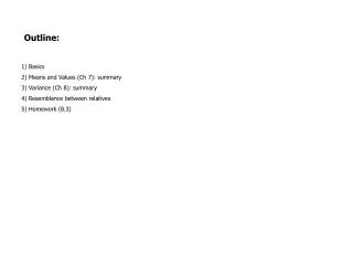
Outline: 1) Basics2) Means and Values (Ch 7): summary3) Variance (Ch 8): summary4) Resemblance between relatives5) Homework (8.3)

Values & means: summary(Falconer & Mackay: chapter 7) Sanja Franic VU University Amsterdam 2011

Summary table: P = G + E = A + D + I+ E

Variance: summary(Falconer & Mackay: chapter 8)

*the more general expression is VP = VG + VE + 2covGE + VGE, where covGE is the covariance between genotypic values and the environmental deviations, and VGE the variance due to interaction between genotypes and the environment.

VA and VD: obtained by squaring the breeding values and dominance deviations, respectively, multiplying by the genotype frequency, and summing over the three genotypes. * Note: As the means of A, G, and D are all 0, no correction for the mean is needed and their variance is obtained simply as the mean of squared values (i.e., in V = Σ(xi- μx)2/N, μx = 0, thus V = Σxi2/N). Given that we work with frequencies, V = Σxi2fi

Resemblance between relatives(Falconer & Mackay: chapter 9)

resemblance between relatives: • one of the basic genetic phenomena displayed by metric traits • easy to determine by simple measurements of the trait • provides the means of estimating the amount of additive genetic variance (VA) • last chapter: causal components of phenotypic variance (V: VE, VG, VA, VD, VI) • observational components of phenptypic variance: s2

resemblance between relatives: • one of the basic genetic phenomena displayed by metric traits • easy to determine by simple measurements of the trait • provides the means of estimating the amount of additive genetic variance (VA) • last chapter: causal components of phenotypic variance (V: VE, VG, VA, VD, VI) • observational components of phenptypic variance: s2 • e.g., grouping of individuals into families of full sibs: • ANOVA: we can partition the total variation into between and within group variance • these components can be used to estimate the covariation between full sibs, as the intraclass correlation coefficient • t = s2B/ (s2B + s2W) • - between group variance (s2B) = covariance of the members of the group → the variance between groups (families) of full sibs = covariance between full sibs • this can be explained in great detail in the next lecture (on heritability)

resemblance between relatives: • one of the basic genetic phenomena displayed by metric traits • easy to determine by simple measurements of the trait • provides the means of estimating the amount of additive genetic variance (VA) • last chapter: causal components of phenotypic variance (V: VE, VG, VA, VD, VI) • observational components of phenptypic variance: s2 • e.g., grouping of individuals into families of full sibs: • ANOVA: we can partition the total variation into between and within group variance • these components can be used to estimate the covariation between full sibs, as the intraclass correlation coefficient: • t = s2B/ (s2B + s2W) • - between group variance (s2B) = covariance of the members of the group → the variance between groups (families) of full sibs = covariance between full sibs • this can be explained in great detail in the next lecture (on heritability) • offspring and parents: • the grouping is in pairs: parent (or mean parent) and offspring (or mean offspring) • the intraclass correlation coefficient (ICC) therefore not necessary (in addition: the phenotypic variance is often not the same in parents and offspring – the sums-of-squares approach is therefore inadequate) • instead, the covariance of offspring with parents is calculated in the standard way (from the sum of cross-products), and standardized as in regression: • covOP = bOP s2P→ bOP = covOP / s2P s2P bOP P O

the phenotypic covariance is composed of the causal components of variance (V) discussed in Ch 8, but in proportions differing according to the sort of relationship • → by finding out how the causal components contribute to the covariance, we will see how the observed covariance can be used to estimate the causal components

the phenotypic covariance is composed of the causal components of variance (V) discussed in Ch 8, but in proportions differing according to the sort of relationship • → by finding out how the causal components contribute to the covariance, we will see how the observed covariance can be used to estimate the causal components • for the time being, we will focus on genetic covariance between relatives (i.e., will not consider the non-genetic covariance) • this means we are considering the covariance between the genotypic values (G) of individuals • assumptions: • Hardy-Weinberg equilibrim • random mating with respect to the trait in question • no epistasis • (these assumptions can be tested, and the effects can be explicitly modeled if the assumptions do not hold)

the phenotypic covariance is composed of the causal components of variance (V) discussed in Ch 8, but in proportions differing according to the sort of relationship • → by finding out how the causal components contribute to the covariance, we will see how the observed covariance can be used to estimate the causal components • for the time being, we will focus on genetic covariance between relatives (i.e., will not consider the non-genetic covariance) • this means we are considering the covariance between the genotypic values (G) of individuals • assumptions: • Hardy-Weinberg equilibrim • random mating with respect to the trait in question • no epistasis • (these assumptions can be tested, and the effects can be explicitly modeled if the assumptions do not hold) • we will consider 4 types of relationships: • parent-offspring • half sibs • full sibs • twins

Offspring and one parent • the covariance of genotypic values of individuals with the mean genotypic value of their offspring (under random mating) • if values are expressed as deviations from the population mean, then the mean value of the offspring is by definition half the breeding value of the parent (Ch 7) • therefore: the covariance in question is the covariance between the genotypic value of an individual with half its breeding value - i.e., the covariance between G and ½A

Offspring and one parent • the covariance of genotypic values of individuals with the mean genotypic value of their offspring (under random mating) • if values are expressed as deviations from the population mean, then the mean value of the offspring is by definition half the breeding value of the parent (Ch 7) • therefore: the covariance in question is the covariance between the genotypic value of an individual with half its breeding value - i.e., the covariance between G and ½A • G = A + D, therefore we are looking at the covariance of A + D with ½A: * • covOP = ( S ½Ai (Ai + Di) ) / N • = (½S Ai (Ai + Di) ) / N • = (½SAi2 + ½SAiDi) ) / N • = ½SAi2/N + ½SAiDi/N • where i (i = 1, …, N) denotes parent-offspring pair. * Note: the variables do not need centering, as they are already expressed as deviations from the population mean

Offspring and one parent • the covariance of genotypic values of individuals with the mean genotypic value of their offspring (under random mating) • if values are expressed as deviations from the population mean, then the mean value of the offspring is by definition half the breeding value of the parent (Ch 7) • therefore: the covariance in question is the covariance between the genotypic value of an individual with half its breeding value - i.e., the covariance between G and ½A • G = A + D, therefore we are looking at the covariance of A + D with ½A: * • covOP = ( S ½Ai (Ai + Di) ) / N • = (½S Ai (Ai + Di) ) / N • = (½SAi2 + ½SAiDi) ) / N • = ½SAi2/N + ½SAiDi/N • where i (i = 1, …, N) denotes parent-offspring pair. • ½SAi2/N = ½VA • ½SAiDi/N = ½covAD • covAD = 0 (from Ch 8) • Therefore: covOP = ½VA→ The genetic covariance between parent and offspring is half the • additive genetic variance of the parents. * Note: the variables do not need centering, as they are already expressed as deviations from the population mean

Offspring and one parent Another way of deriving the covariance: A2A2 A1A2 A1A1 Genotype Genotypic values (a, d, -a) expressed as deviations from the population mean Genotypicvalue - a 0 d + a Genotype frequency q2 2pq p2

Offspring and one parent Another way of deriving the covariance: A2A2 A1A2 A1A1 Genotype Genotypic values (a, d, -a) expressed as deviations from the population mean Genotypicvalue - a 0 d + a a – m = a – [(p – q) + 2dpq] = 2q(a - qd) m

Offspring and one parent Another way of deriving the covariance: mean cross-product of these

Offspring and one parent Another way of deriving the covariance: covOP = 2q2p2a(a – qd) + pqa(q – p) [(q – p)a + 2qpd] + 2p2q2a(a + pd) = pqa2 = ½VA, since VA = 2pqa2. covOP = bOP * VP bOP = covOP / VP = ½VA / VP mean cross-product of these VP bOP P O

Offspring and mid-parent • mid-parent = mean of the two parents • O = mean genotypic value of the offspring • P & P’ = genotypic values of the two parents • mid-parent genotypic value: P = ½(P + P’) • covOP = SOP/N • = S½(P + P’)O / N • = (½SPO + ½SP’O) / N • = ½SPO/N + ½SP’O/N • = ½covOP + ½covOP’ • If the P and P’ have the same variance, then covOP = covOP’, so: • covOP= covOP = ½VA → Therefore the covariance is the same as in the case of offspring and one parent

Offspring and mid-parent • mid-parent = mean of the two parents • O = mean genotypic value of the offspring • P & P’ = genotypic values of the two parents • mid-parent genotypic value: P = ½(P + P’) • covOP = SOP/N • = S½(P + P’)O / N • = (½SPO + ½SP’O) / N • = ½SPO/N + ½SP’O/N • = ½covOP + ½covOP’ • If the P and P’ have the same variance, then covOP = covOP’, so: • covOP= covOP = ½VA → Therefore the covariance is the same as in the case of offspring and one parent • However, the regression coefficient is different. The variance of the mean of n variables is 1/n of variance of single variables. Therefore, VP = ½VP. • bOP = covOP / ½VP • = ½VA / ½VP = VA/VP ½VP bOP P O

Half sibs • a group of half sibs = progeny of one individual mated to a random group of the other sex, having one offspring by each mate • therefore, by definition, the mean genotypic value of a group of half sibs is half the breeding value of the common parent • the covariance of half sibs is the variance of the true values of the half-sib groups (i.e., it is the between-group variance; will be explained more in the lecture on ICC) • the true mean of each half sib group is half the breeding value of the parent • therefore, the covariance of half sibs is the variance of is half the breeding value of the parent, which is a quarter of the additive variance (trust me, or should I derive it?): • covHS = V½A = ¼VA

If you wanted me to derive it:

Half sibs • a group of half sibs = progeny of one individual mated to a random group of the other sex, having one offspring by each mate • therefore, by definition, the mean genotypic value of a group of half sibs is half the breeding value of the common parent • the covariance of half sibs is the variance of the true values of the half-sib groups (i.e., it is the between-group variance; will be explained more in the lecture on ICC) • the true mean of each half sib group is half the breeding value of the parent • therefore, the covariance of half sibs is the variance of is half the breeding value of the parent, which is a quarter of the additive variance (trust me, or should I derive it?): • covHS= V½A = ¼VA • degree of resemblance between half sibs is expressed as the ICC (the between group variance [i.e., the covariance] as a proportion of total variance): • t = ¼VA/VP

Full sibs • dominance variance contributes to the covariance between full sibs (unlike the relationships considered so far) • additive variance: • full sibs share both parents; therefore, their mean genotypic value equals the mean breeding value of the two parents • therefore, the covariance is the variance of ½(A + A’) • var½(A + A’) = ¼(VA + VA’) • = ½VAif the additive genetic variance is equal in the two sexes.

Full sibs • dominance variance contributes to the covariance between full sibs (unlike the relationships considered so far) • additive variance: • full sibs share both parents; therefore, their mean genotypic value equals the mean breeding value of the two parents • therefore, the covariance is the variance of ½(A + A’) • var½(A + A’) = ¼(VA + VA’) • = ½VAif the additive genetic variance is equal in the two sexes. • dominance variance: • let parents have genotypes A1A2 and A3A4 • then there are 4 genotypes in the progeny: A1A3, A1A4, A2A3, A2A4, each with a frequency of ¼ • let one of the sibs have any of the genotypes • then the probability that the other sib will have the same genotype is ¼ • therefore, ¼ of full sibs have the same genotype, and consequently the same dominance deviation, D • for these pairs, the cross-product of dominance deviations is D2 • for other pairs, this cross-product is 0 • therefore, on average, the (mean) cross-product is ¼SD2 / N, which equals ¼VD • total genetic covariance of full sibs is therefore: • covFS = ½VA + ¼VD

Full sibs • the correlation of full sibs is: • t = (½VA + ¼VD) / VP

Twins • - dizygotic (DZ) twins are related as full sibs; their genetic covariance is that of full sibs: • covDZ = ½VA + ¼VD • monozygotic (MZ) twins have identical genotypes, therefore: • covMZ = VG

Environmental covariance • related individuals may resemble each other for environmental reasons as well (some relatives more than others) • family members reared together share a common environment -> some environmental circumstances that cause differences between unrelated individuals are not a cause of difference between members of the same family • -> there is a component of environmental variance that contributes to the variance between means of families, but not to the variance within families -> therefore, it contributes to the covariance of family members • this components is termed VEc: common environment • the remainder of environmental variance (VEw) arises from causes of difference that are unconnected to whether the individuals are related or not • therefore, VEw appears in the within-group component of variance, but does not contribute to the between-group component • the total environmental variance can therefore be partitioned as follows: • VE = VEc + VEw, • where the VEc component contributes to the covariance of related invididuals.

Summary

Applications in structural equation modeling

Homework 9.3 (you’ll need to read Ch 9 to understand the solution, pleasebeable to explain it in class)

Values & means: summary (Falconer & Mackay: chapter 7)