Download

1 / 97
1.01k likes | 1.41k Views
4.1 Extreme Values of Functions. Absolute extreme values are either maximum or minimum points on a curve. They are sometimes called global extremes. They are also sometimes called absolute extrema . ( Extrema is the plural of the Latin extremum .). 4.1 Extreme Values of Functions.

E N D
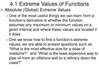
4.1 Extreme Values of Functions Absolute extreme values are either maximum or minimum points on a curve. They are sometimes called global extremes. They are also sometimes called absolute extrema. (Extrema is the plural of the Latin extremum.)
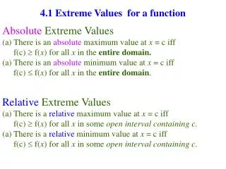
4.1 Extreme Values of Functions • DefinitionAbsolute Extreme Values • Let f be a function with domain D. Then f (c) is the • absolute minimum value on D if and only • if f(x) <f (c) for all x in D. • absolute maximum value on D if and only • if f(x) >f (c) for all x in D.
4.1 Extreme Values of Functions Extreme values can be in the interior or the end points of a function. No Absolute Maximum Absolute Minimum
4.1 Extreme Values of Functions Absolute Maximum Absolute Minimum
4.1 Extreme Values of Functions Absolute Maximum No Minimum
4.1 Extreme Values of Functions No Maximum No Minimum
4.1 Extreme Values of Functions Extreme Value Theorem: If f is continuous over a closed interval, [a,b] then f has a maximum and minimum value over that interval. Maximum at interior point, minimum at endpoint Maximum & minimum at interior points Maximum & minimum at endpoints
4.1 Extreme Values of Functions Local Extreme Values: A local maximum is the maximum value within some open interval. A local minimum is the minimum value within some open interval.
4.1 Extreme Values of Functions Local extremes are also called relative extremes. Absolute maximum (also local maximum) Local maximum Local minimum Local minimum Absolute minimum (also local minimum)
4.1 Extreme Values of Functions Notice that local extremes in the interior of the function occur where is zero or is undefined. Absolute maximum (also local maximum) Local maximum Local minimum
4.1 Extreme Values of Functions Local Extreme Values: If a function f has a local maximum value or a local minimum value at an interior point c of its domain, and if exists at c, then
4.1 Extreme Values of Functions Critical Point: A point in the domain of a function f at which or does not exist is a critical point of f . Note: Maximum and minimum points in the interior of a function always occur at critical points, but critical points are not always maximum or minimum values.
4.1 Extreme Values of Functions EXAMPLE 3FINDING ABSOLUTE EXTREMA Find the absolute maximum and minimum values of on the interval . There are no values of x that will make the first derivative equal to zero. The first derivative is undefined at x=0, so (0,0) is a critical point. Because the function is defined over a closed interval, we also must check the endpoints.
4.1 Extreme Values of Functions At: At: At: To determine if this critical point is actually a maximum or minimum, we try points on either side, without passing other critical points. Since 0<1, this must be at least a local minimum, and possibly a global minimum.
4.1 Extreme Values of Functions Absolute minimum: Absolute maximum: At: At:
4.1 Extreme Values of Functions y = x2/3
4.1 Extreme Values of Functions 1 4 Find the derivative of the function, and determine where the derivative is zero or undefined. These are the critical points. For closed intervals, check the end points as well. 2 Find the value of the function at each critical point. 3 Find values or slopes for points between the critical points to determine if the critical points are maximums or minimums. Finding Maximums and Minimums Analytically:
4.1 Extreme Values of Functions Find the absolute maximum and minimum of the function Find the critical numbers
4.1 Extreme Values of Functions Find the absolute maximum and minimum of the function Check endpoints and critical numbers The absolute maximum is 2 when x = -2 The absolute minimum is -13 when x = -1
4.1 Extreme Values of Functions Find the absolute maximum and minimum of the function Find the critical numbers
4.1 Extreme Values of Functions Find the absolute maximum and minimum of the function Check endpoints and critical numbers The absolute maximum is 3 when x = 0, 3 The absolute minimum is 2 when x = 1
4.1 Extreme Values of Functions Find the absolute maximum and minimum of the function Find the critical numbers
4.1 Extreme Values of Functions Find the absolute maximum and minimum of the function The absolute maximum is 1/4 when x = /6, 5/6 The absolute minimum is –2 when x =3/2
4.1 Extreme Values of Functions Critical points are not always extremes! (not an extreme)
4.1 Extreme Values of Functions (not an extreme)
4.2 Mean Value Theorem Mean Value Theorem for Derivatives If f (x) is a differentiable function over [a,b], then at some point between a and b:
4.2 Mean Value Theorem If f (x) is a differentiable function over [a,b], then at some point between a and b: Mean Value Theorem for Derivatives Differentiable implies that the function is also continuous.
4.2 Mean Value Theorem If f (x) is a differentiable function over [a,b], then at some point between a and b: Mean Value Theorem for Derivatives Differentiable implies that the function is also continuous. The Mean Value Theorem only applies over a closed interval.
4.2 Mean Value Theorem If f (x) is a differentiable function over [a,b], then at some point between a and b: The Mean Value Theorem says that at some point in the closed interval, the actual slope equals the average slope. Mean Value Theorem for Derivatives
4.2 Mean Value Theorem Tangent parallel to chord. Slope of tangent: Slope of chord:
4.2 Mean Value Theorem (b,0) (a,0) Rolle’s Theorem If f (x) is a differentiable function over [a,b], and if f(a) = f(b) = 0, then there is at least one point c between a and b such that f’(c)=0:
4.2 Mean Value Theorem Show the function satisfies the hypothesis of the Mean Value Theorem The function is continuous on [0,/3] and differentiable on (0,/3). Since f(0) = 1 and f(/3) = 1/2, the Mean Value Theorem guarantees a point c in the interval (0,/3) for which c = .498
4.2 Mean Value Theorem (0,1) at x = .498, the slope of the tangent line is equal to the slope of the chord. (/3,1/2)
4.2 Mean Value Theorem • Definitions Increasing Functions, Decreasing Functions • Let f be a function defined on an interval I and let x1 and x2 • be any two points in I. • f increases on I if x1 < x2 f(x1) < f(x2). • f decreases on I if x1 > x2 f(x1) > f(x2).
4.2 Mean Value Theorem A function is increasing over an interval if the derivative is always positive. A function is decreasing over an interval if the derivative is always negative. • Corollary Increasing Functions, Decreasing Functions • Let f be continuous on [a,b] and differentiable on (a,b). • If f’ > 0 at each point of (a,b), then f increases on [a,b]. • If f’ < 0 at each point of (a,b), then f decreases on [a,b]. A couple of somewhat obvious definitions:
- + + 0 0 f’(x) 2 4 4.2 Mean Value Theorem Find where the function is increasing and decreasing and find the local extrema. x = 2, local maximum x = 4, local minimum
(2,20) local max (4,16) local min 4.2 Mean Value Theorem
4.2 Mean Value Theorem Functions with the same derivative differ by a constant. These two functions have the same slope at any value of x.
4.2 Mean Value Theorem Find the function whose derivative is and whose graph passes through so:
4.2 Mean Value Theorem Find the function f(x) whose derivative is sin(x) and whose graph passes through (0,2). so: Notice that we had to have initial values to determine the value of C.
4.2 Mean Value Theorem Antiderivative A function is an antiderivative of a function if for all x in the domain of f. The process of finding an antiderivative is antidifferentiation. The process of finding the original function from the derivative is so important that it has a name: You will hear much more about antiderivatives in the future. This section is just an introduction.
4.2 Mean Value Theorem Example 7b: Find the velocity and position equations for a downward acceleration of 9.8 m/sec2 and an initial velocity of 1 m/sec downward. (We let down be positive.) Since acceleration is the derivative of velocity, velocity must be the antiderivative of acceleration.
4.2 Mean Value Theorem The power rule in reverse: Increase the exponent by one and multiply by the reciprocal of the new exponent. Since velocity is the derivative of position, position must be the antiderivative of velocity.
4.2 Mean Value Theorem The initial position is zero at time zero.
4.3 Connecting f’ and f’’ with the Graph of f In the past, one of the important uses of derivatives was as an aid in curve sketching. We usually use a calculator of computer to draw complicated graphs, it is still important to understand the relationships between derivatives and graphs.
4.3 Connecting f’ and f’’ with the Graph of f local max f’>0 f’<0 local min f’>0 f’<0 no extreme f’>0 f’>0 First Derivative Test for Local Extrema at a critical point c • If f ‘changes sign from positive to • negative at c, then f has a local • maximum at c. 2. If f ‘ changes sign from negative to positive at c, then f has a local minimum at c. • If f ‘ changes does not change sign • at c, then f has no local extrema.
4.3 Connecting f’ and f’’ with the Graph of f is positive is negative is zero First derivative: Curve is rising. Curve is falling. Possible local maximum or minimum.
4.3 Connecting f’ and f’’ with the Graph of f concave up concave down • DefinitionConcavity • The graph of a differentiable • function y = f(x) is • concave up on an open interval • I if y’ is increasing on I. (y’’>0) • concave down on an open interval • I if y’ is decreasing on I. (y’’<0)
4.3 Connecting f’ and f’’ with the Graph of f + + • Second Derivative Test for Local Extrema at a critical point c • If f’(c) = 0 and f’’(c) < 0, then f has a local maximum at x = c. • If f’(c) = 0 and f’’(c) > 0, then f has a local minimum at x = c.
4.3 Connecting f’ and f’’ with the Graph of f is positive is negative is zero Second derivative: Curve is concave up. Curve is concave down. Possible inflection point (where concavity changes).