Faster least squares approximation
Faster least squares approximation. Tamas Sarlos Yahoo! Research IPAM 23 Oct 2007 http://www.ilab.sztaki.hu/~stamas Joint work with P. Drineas, M. Mahoney, and S. Muthukrishnan. Outline. Randomized methods for Least squares approximation Lp regression Regularized regression

Faster least squares approximation
E N D
Presentation Transcript
Faster least squares approximation Tamas Sarlos Yahoo! Research IPAM 23 Oct 2007 http://www.ilab.sztaki.hu/~stamas Joint work with P. Drineas, M. Mahoney, and S. Muthukrishnan.
Outline Randomized methods for • Least squares approximation • Lp regression • Regularized regression • Low rank matrix approximation
Models, curve fitting, and data analysis In MANY applications (in statistical data analysis and scientific computation), one has n observations (values of a dependent variable y measured at values of an independent variable t): Model y(t) by a linear combination of d basis functions: A is an n x d “design matrix” with elements: In matrix-vector notation:
Least Squares (LS) Approximation We are interested in over-constrained L2 regression problems, n >> d. Typically, there is no x such that Ax = b. Want to find the “best” x such that Ax ≈ b. Ubiquitous in applications & central to theory: Statistical interpretation: best linear unbiased estimator. Geometric interpretation: orthogonally project b onto span(A).
Many applications of this! • Astronomy: Predicting the orbit of the asteroid Ceres (in 1801!). Gauss (1809) -- see also Legendre (1805) and Adrain (1808). First application of “least squares optimization” and runs in O(nd2) time! • Bioinformatics: Dimension reduction for classification of gene expression microarray data. • Medicine: Inverse treatment planning and fast intensity-modulated radiation therapy. • Engineering: Finite elements methods for solving Poisson, etc. equation. • Control theory: Optimal design and control theory problems. • Economics: Restricted maximum-likelihood estimation in econometrics. • Image Analysis: Array signal and image processing. • Computer Science: Computer vision, document and information retrieval. • Internet Analysis: Filtering and de-noising of noisy internet data. • Data analysis: Fit parameters of a biological, chemical, economic, social, internet, etc. model to experimental data.
Projection of b on the subspace spanned by the columns of A Pseudoinverse of A Exact solution to LS Approximation Cholesky Decomposition: If A is full rank and well-conditioned, decompose ATA = RTR, where R is upper triangular, and solve the normal equations: RTRx=ATb. QR Decomposition: Slower but numerically stable, esp. if A is rank-deficient. Write A=QR, and solve Rx = QTb. Singular Value Decomposition: Most expensive, but best if A is very ill-conditioned. Write A=UVT, in which case: xOPT = A+b = V-1kUTb. Complexity is O(nd2) for all of these, but constant factors differ.
Reduction of LS Approximation to fast matrix multiplication Theorem: For any n-by-d matrix A, and d dimensional vector b, where n>d, we can compute x*=A+b in O(n/dM(d)) time. Here M(d) denotes the time needed to multiply two d-by-d matrices. • Current best M(d)=d, =2.376… Coppersmith–Winograd (1990) Proof: Ibarra et al. (1982) generalize the LUP decomposition for rectangular matrixes Direct proof: • Recall the normal equations ATAx = ATb • Group the rows of A into blocks of d and compute ATA as the sum of n/d square products, each d-by-d • Solve the normal equations • LS in O(nd1.376) time, but impractical. We assume O(nd2).
Original (expensive) sampling algorithm Drineas, Mahoney, and Muthukrishnan (SODA, 2006) • Algorithm • Fix a set of probabilities pi, i=1,…,n. • Pick the i-th row of A and the i-th element of b with probability • min {1, rpi}, • and rescale by (1/min{1,rpi})1/2. • Solve the induced problem. Theorem: Let: If the pi satisfy: for some (0,1], then w.p. ≥ 1-, • These probabilities pi’s are statistical leverage scores! • “Expensive” to compute, O(nd2) time, these pi’s!
Fast LS via uniform sampling Drineas, Mahoney, Muthukrishnan, and Sarlos (2007) • Algorithm • Pre-process A and b with a “randomized Hadamard transform”. • Uniformly sample • r=O(d log(n) log(d log(n))/) • constraints. • Solve the induced problem: • Non-uniform sampling will work, but it is “slow.” • Uniform sampling is “fast,” but will it work?
A structural lemma Approximate by solving where is any matrix. Let be the matrix of left singular vectors of A. assume that -fraction of mass of b lies in span(A). Lemma: Assume that: Then, we get relative-error approximation:
Randomized Hadamard preprocessing Facts implicit or explicit in: Ailon & Chazelle (2006), or Ailon and Liberty (2008). Let Hn be an n-by-n deterministic Hadamard matrix, and Let Dn be an n-by-n random diagonal matrix with +1/-1 chosen u.a.r. on the diagonal. Fact 1: Multiplication by HnDn doesn’t change the solution: (since Hn and Dn are orthogonal matrices). Fact 2: Multiplication by HnDn is fast - only O(n log(r)) time, where r is the number of elements of the output vector we need to “touch”. Fact 3: Multiplication by HnDn approximately uniformizes all leverage scores:
Establishing structural conditions Lemma: |1-i2(SHUA)| ≤ 1/10, with constant probability, i.e,. singular values of SHUA are close to 1. Proof: Apply spectral norm matrix perturbation bound. Lemma: ||(SHUA)TSHb|| ≤ OPT, with constant probability, i.e., SHUA is nearly orthogonal to b. Proof: Apply Forbenius norm matrix perturbation bound. Bottom line: • Fast algorithm approximately uniformizes the leverage of each data point. • Uniform sampling is optimal up to O(1/log(n)) factor, so over-sample a bit. • Overall running time O(ndlog(…)+d3log(…)/)
Fast LS via sparse projection Drineas, Mahoney, Muthukrishnan, and Sarlos (2007) - sparse projection matrix from Matousek’s version of Ailon-Chazelle 2006 • Algorithm • Pre-process A and b with a randomized Hadamard transform. • Multiply preprocessed input by sparse random k x n matrix T, where • and where k=O(d/) and q=O(d log2(n)/n+d2log(n)/n) . • Solve the induced problem: • Dense projections will work, but it is “slow.” • Sparse projection is “fast,” but will it work? • -> YES! Sparsity parameter q of T related to non-uniformity of leverage scores!
Lp regression problems Dasgupta, Drineas, Harb, Kumar, and Mahoney (2008) We are interested in over-constrained Lp regression problems, n >> d. Lp regression problems are convex programs (or better!). There exist poly-time algorithms. We want to solve them faster!
Lp norms and their unit balls Recall the Lp norm for : Some inequality relationships include:
Solution to Lp regression Lp regression can be cast as a convex program for all . For p=1, Sum of absolute residuals approximation (minimize ||Ax-b||1): For p=∞, Chebyshev or mini-max approximation (minimize ||Ax-b||∞): For p=2, Least-squares approximation (minimize ||Ax-b||2):
What made the L2 result work? • The L2 sampling algorithm worked because: • For p=2, an orthogonal basis (from SVD, QR, etc.) is a “good” or “well-conditioned” basis. • (This came for free, since orthogonal bases are the obvious choice.) • Sampling w.r.t. the “good” basis allowed us to perform “subspace-preserving sampling.” • (This allowed us to preserve the rank of the matrix and distances in its span.) • Can we generalize these two ideas to p2?
Sufficient condition Easy Approximate minx||b-Ax||p by solving minx||S(b-Ax)||p giving x’ Assume that the matrix S is an isometry over the span of A and b: for any vector y in span(Ab) we have (1-)||y||p ||Sy||p (1+ ) ||y|| p Then, we get relative-error approximation: ||b-Ax||p (1+ ) minx|| S(b-Ax)||p (This requires O(d/2) for L2 regression.) How to construct an Lp isometry?
p-well-conditioned basis (definition) Let A be an n x m matrix of rank d<<n, let p [1,∞), and q its dual. Definition: An n x d matrix U is an (,,p)-well-conditioned basis for span(A) if: (1) |||U|||p≤, (where |||U|||p = (ij|Uij|p)1/p ) (2) for all z in Rd, ||z||q ≤ ||Uz||p. U is a p-well-conditioned basis if ,=dO(1), independent of m,n.
p-well-conditioned basis (existence) Let A be an n x m matrix of rank d<<n, let p [1,∞), and q its dual. Theorem: There exists an (,,p)-well-conditioned basis U for span(A) s.t.: if p < 2, then = d1/p+1/2 and = 1, if p = 2, then = d1/2and = 1, if p > 2, then = d1/p+1/2and = d1/q-1/2. U can be computed in O(nmd+nd5log n) time (or just O(nmd) if p = 2).
p-well-conditioned basis (construction) • Algorithm: • Let A=QR be any QR decomposition of A. • (Stop if p=2.) • Define the norm on Rd by ||z||Q,p ||Qz||p. • Let C be the unit ball of the norm ||•||Q,p. • Let the d x d matrix F define the Lowner-John ellipsoid of C. • Decompose F=GTG, • where G is full rank and upper triangular. • Return U = QG-1 • as the p-well-conditioned basis.
Subspace-preserving sampling Let A be an n x m matrix of rank d<<n, let p [1,∞). Let U be an (,,p)-well-conditioned basis for span(A), Theorem: Randomly sample rows of A according to the probability distribution: where: Then, with probability 1- , the following holds for all x in Rm:
Regularized regression • If you don’t trust your data (entirely) • Minimize ||b-Ax||p+||x||r, where r arbitrary • Lasso is especially popular: minx||b-Ax||2+||x||1 • Sampled Lp regression works for the regularized version too • We want more: imagine
Ridge regression • Tikhonov regularization, back to L2 • Minimize ||b-Ax||22+2||x||22 • Equivalent to augmenting n-by-d A with dand b with 0 • SVD of A UDiag(sqrt(i))VT • Let D = i sqrt(i) << d • For (1+)relative error: • precondition with randomized FFT • sample r=O(D log(n) log(D log(n))/) rows uniformly.
SVD of a matrix Any m x n matrix A can be decomposed as: U (V): orthogonal matrix containing the left (right) singular vectors of A. S: diagonal matrix containing the singular values of A, ordered non-increasingly. : rank of A, the number of non-zero singular values. Exact computation of the SVD takes O(min{mn2 , m2n}) time.
SVD and low-rank approximations Truncate the SVD by keeping k ≤ terms: • Uk (Vk): orthogonal matrix containing the top k left (right) singular vectors of A. • k: diagonal matrix containing the top k singular values of A. • Ak is the “best” matrix among all rank-k matrices wrt. to the spectral and Frobenius norms • This optimality property of very useful in, e.g., Principal Component Analysis (PCA), LSI, etc.
Approximate SVD • Starting with the seminal work of Frieze et al (1998) • and Papadimitriou et al (1998) till 2005 several results • of the form • ||A-Ak’||F ≤ ||A-Ak||F + t||A||F • ||A||F might be a significantly larger than ||A-Ak||F • Four independent results [H-P, DV, MRT, S 06] on • ||A-Ak’||F ≤ (1+)||A-Ak||F • This year Shyanalkumar and Deshpande …
Relative error SVD via random projections • Theorem Let S be n by r=O(k/) random matrix with • 1 entries. Project A to the subspace spanned by the rows of SA and then compute Ak’ as • the rank-k SVD of the projection. Then • ||A-Ak’||F ≤ (1+)||A-Ak||F with prob. at least 1/3 • By keeping an orthonormal basis of SA total time is O(Mr+(n+m)r^2) with M non-zeroes • We need to make only 2 passes over the data • Can use fast random projections and avoid the SA projection, spectral norm (talks by R and T)
SVD proof sketch Can show: ||A-Ak’||F2 ≤ ||A-Ak||F2 + ||Ak-Ak(SAk)+(SA)||F2 For all j columns of A consider the regression A(j)≈Akx Exact: Ak(j), error is ||A(j)-Ak(j)||2 Approximate: Ak-Ak(SAk)+SA(j)
Conclusion Fast methods based on randomized preprocessing and sampling or sparse projections for • Least squares approximation • Regularized regression • Low rank matrix approximation