Download
1 / 22
230 likes | 388 Views
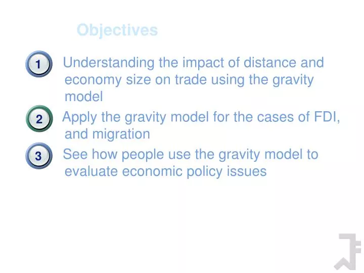
1. 3. 2. Objectives. Understanding the impact of distance and economy size on trade using the gravity model Apply the gravity model for the cases of FDI, and migration See how people use the gravity model to evaluate economic policy issues. The Origin of the Gravity Equation.

E N D
1 3 2 Objectives Understanding the impact of distance and economy size on trade using the gravity model Apply the gravity model for the cases of FDI, and migration See how people use the gravity model to evaluate economic policy issues
The Origin of the Gravity Equation • Newton’s “Law of Universal Gravitation” (1687): The attractive force (Fij) between i and j • Mi, Mj are the masses • D is distance between two objects • G is gravitational constant Mi Mj F D
Economists and Gravity • Model many social interactions (migration, tourism, trade, FDI) • Fij is the flow from i to j • M’s are measure of economic mass • D is the distance
Estimation of the Gravity Equation • Take logs:
Overall explanatory power • R2 between 0.65 and 0.95 • Suggests using gravity as a benchmark for volume of trade. • Can then use gravity based benchmark to evaluate economic policy
The role of economic mass • Usually measured using GDP • Most theoretical explanations predict coefficient equal to one • Estimates often not significantly different from 1, but range is from 0.7 to 1.1
The role of distance • Distance usually measured using great circle distance based on latitude and longitude • Head (2000) averages results from 62 regressions in eight papers, for sample years ranging from 1928 to 1995 • Average distance effect is 1.01 • Doubling distance halves trade
Distance and trade costs • Trade costs: • Direct (transport) • Indirect (government policy; language) • Is distance just capturing the effect of trade costs (acting as a proxy) or does it play an additional role?
Data on trade costs • IMF bilateral data of total exports from A (free on board) to imports of B (cost-insurance-freight) • Composition of trade depends on t.c. • National customs data for a few countries • Direct industry/shipping company info • Ocean shipping prices/air freight from trade journals (Hummels) • Quotes from shipping standard container from Baltimore (Venables)
Magnitude • Wide dispersion of trade costs • US 3.8% value of imports (1994) • Brazil 7.3% • Paraguay 13.3% • Unweighted (get rid of composition effect) • Median cif/fob ratio 1.28 (28% t.c.) • 2 to 3 times higher than weighted
Effect of distance on t.c. • Mean cost if not landlocked $4,620 • Landlocked increases cost by $3,450 • Overland 7 times more expensive than sea • For cif/fob ratios • Elasticity w.r.t distance 0.2 to 0.3 • Common border reduces substantially • R2 = 0.45
Distance and gravity • Distance explains around 45% variation in transport costs • Regressions of trade flows on both distance and t.c. still gives significant coefficient on distance (although magnitude lower) • Distance must be a proxy for both t.c. and other information costs.
Using gravity to test for border effects. • Home bias: preference towards home products; • Comparison between intranational trade and international trade; • The borderless world – “National borders have effectively disappeared” • Use gravity to test: • McCallum (1995) using data on trade flows between US and Canadian provinces (dummy=1 if in the same country)
Using gravity to test for border effects. • McCallum: Data referring to 1988 (before FTA Canada-USA was signed): Intra-national data flows only referred to Canada (exports from a province to other Canada provinces: DumCA=1); International: Exports from Canada provinces to USA states (DumCA=0) • Developments: addiction of data referring to 1993: intra-national data for both CA and USA. Another indicator=DumUSA=1 for trade between two USA states; • Dij is the distance between any two provinces or states; • Results
Using gravity to test for border effects. • Data referring to 1988 (before FTA Canada-USA was signed): Intra-national data flows only referred to Canada (exports from a province to other Canada provinces: Dummy=1); International: Exports from Canada provinces to USA states (Dummy=0) • Data referring to 1993: intra-national data for both CA and USA • Dij is the distance between any two provinces or states; • Results
The importance of borders • 1988 or 1993: Coefficient on cross-provincial trade is quite high (3.09 to 2.75). Exp(3.09)=22; Exp(2.75)=15.7 • 1988: Canada-Canada province trade approx. 22 times Canada-US state trade; 1993: reduced to 15,7 • Border effects (all impediments to trade across borders) • Ontario’s shipments to British Columbia should be 0.6 times shipments to Washington (US) [Washington is richer] • BC receives 12.6 times more goods from Ontario than Washington • Border effect = 12.6/0.6 = 21 • Fallen to 12 since FTA implemented
The importance of borders • Anderson and Wincoop (2003): border effects have an asymmetric effect on countries of different size. More precisely have a larger effect on small economies. • Example: • US is 10 times bigger than Canada (economic size) • Without frictions to trade, Canada exports 90% of its GDP to US and sells 10% internally; US exports 10% of GDP • Suppose border effects reduce trade of a factor of ½ • => Canada exports 45% to US and sells internally 55% • Its internal trade has increased of a factor 5.5, cross-border has decreased by 0.5 => 5.5/0.5=11: internal trade has increased 11 times more than cross-border trade • =>US exports now 5% and sells internally 95%. Cross-state trade has increased only slightly more than 2 times cross-border trade
Alternative approach: taking into account of different prices in different countries • Anderson and Wincoop (2003): • Imposes restrictions on the parameters of M; • Inverse indicator: DUMMY=1 for international (cross-border) trade 0 for internal trade; No distinction between Canadian or US cross-border trade (under a following assumption); • Introduces 2 new variables: price terms of the two countries (whose difference has a meaning). The two variables can be: • Constructed from Price Indexes data; • Estimated as a function of trade costs, where trade costs are a function of distance and other factors (intercept). (N.B. If trade costs are symmetric, then there cannot be a distinction between Canadian and US trade) => this methodology is quite complicated, because it involves the estimation of a recursive model of multiple equations.
Alternative approach: taking into account of different prices in different countries • Anderson and Wincoop (2003): 3. Introduce fixed-effects: two dummies one for the origin country and another one for the destination country: Di=1 if i is the exporter, 0 otherwise; Dj=1 if j is the importer, 0 otherwise; The two dummies are both equal to 1 only for cross-border trade observations. This implies: Di=(1-s)lnPi and Dj=(1-s)lnPj
Conclusions • Distance matters for trade • Consistent with both new trade theory and old trade theory • Theory has helped refine the gravity relationship • Gravity can be used to test other hypotheses even if we don’t know what drives gravity