Download
1 / 26
260 likes | 400 Views
ATMO 336 Weather, Climate and Society Surface and Upper-Air Maps. N. Pacific Pressure Analysis (isobars every 4 mb). 2000 km. Pressure varies by 1 mb per 100 km horizontally or 0.0001 mb per 10 m. Review: Pressure-Height. Remember…

E N D
ATMO 336Weather, Climate and SocietySurface and Upper-Air Maps
N. Pacific Pressure Analysis (isobars every 4 mb) 2000 km Pressure varies by 1 mb per 100 km horizontally or 0.0001 mb per 10 m
Review: Pressure-Height Remember… Pressure falls very rapidly with height near sea-level 3,000 m 701 mb 2,500 m 747 mb 2,000 m 795 mb 1,500 m 846 mb 1,000 m 899 mb 500 m 955 mb 0 m 1013 mb 1 mb per 10 m height Consequently……….Vertical pressure changes from differences in station elevation dominate horizontal changes
Station Pressure Ahrens, Fig. 6.7 Pressure is recorded at stations with different altitudes Station pressure differences reflect altitude differences Wind is forced by horizontal pressure differences Since horizontal pressure variations are 1 mb per 100 km We must adjust station pressures to one standard level: Mean Sea Level
Reduction to Sea-Level-Pressure Ahrens, Fig. 6.7 Station pressures are adjusted toSea Level PressureMake altitude correction of 1 mb per 10 m elevation
Summary • Because horizontal pressure differences are the force that drives the wind Station pressures are adjusted to one standard level…Mean Sea Level…to remove the dominating impact of different elevations on pressure change
Correction for Tucson Elevation of Tucson AZ is ~800 m Station pressure at Tucson runs ~930 mb So SLP for Tucson would be SLP = 930 mb + (1 mb / 10 m)x800 m SLP = 930 mb + 80 mb = 1010 mb
Correction for Denver Elevation of Denver CO is ~1600 m Station pressure at Denver runs ~850 mb So SLP for Denver would be SLP = 850 mb + (1 mb / 10 m)x1600 m SLP = 850 mb + 160 mb = 1010 mb Actual pressure corrections take into account temperature and pressure-height variations, but 1 mb / 10 m is a good approximation
Lets Try for Phoenix Elevation of Phoenix AZ is ~340 m Assume station pressure at PHX is ~977 mb What would the SLP for PHX be?
Correction for Phoenix Elevation of PHX Airport is ~340 m Station pressure at PHX is ~977 mb So, SLP for PHX would be SLP =977 mb + (1 mb / 10 m)x340 m SLP =977 mb + 34 mb = 1011 mb
Local Example Station pressure at PHX is ~977 mb. Station pressure at TUS is ~932 mb. Which station has that higher SLP?
Correction for Tucson Elevation of TUS Airport is ~800 m Station pressure at TUS was ~932 mb So, SLP for TUS would be SLP =932 mb + (1 mb / 10 m)x800 m SLP =932 mb + 80 mb = 1012 mb PHX (prior slide) has SLP = 1011 mb Thus, the SLP was higher in TUS than PHX
Sea Level Pressure Values 882 mb (26.04 in.) Wilma (October, 2005) Ahrens, Fig. 6.3
Summary • Because horizontal pressure differences are the force that drives the wind Station pressures are adjusted to one standard level…Mean Sea Level…to mitigate the impact of different elevations on pressure
PGF Ahrens, Fig. 6.7
Surface Maps • Pressure reduced to Mean Sea Level is plotted and analyzed for surface maps. Estimated from station pressures • Actual surface observations for other weather elements (e.g. temperatures, dew points, winds, etc.) are plotted on surface maps. • NCEP/HPC Daily Weather Map • UIUC 2010 Surface Maps
Winds blow from high to low pressure. Station Plot Explanation
Force of Friction 1 Pressure Gradient Force 1004 mb Friction Geostrophic Wind 1008 mb Coriolis Force Frictional Force is directed opposite to velocity. It acts to slow down (decelerate) the wind. As the wind speed becomes slower, the Coriolis Force would also decrease.
Force of Friction 1 Pressure Gradient Force 1004 mb Friction Geostrophic Wind 1008 mb Coriolis Force Coriolis force no longer can balance the larger Pressure Gradient Force, so the parcel will accelerate since the net force is not zero. Geostrophic balance is no longer possible!
Force of Friction 2 Pressure Gradient Force 1004 mb Wind Friction 1008 mb Coriolis Force Because PGF is larger than CF, air parcel will turn toward lower pressure. Friction Turns Wind Toward Lower Pressure.
Force of Friction 3 1004 mb Wind CF PGF 1008 mb Fr Eventually, a balance among the PGF, Coriolis and Frictional Force is achieved. PGF + CF + Friction = 0 Net force is zero, so parcel does not accelerate.
Force of Friction 4 1004 mb 30o-40o Mtns Water 20o-30o 1008 mb The decrease in wind speed and deviation to lower pressure depends on surface roughness. Smooth surfaces (water) show the least slowing and turning (typically 20o-30o from geostrophic). Rough surfaces (mtns) show the most slowing and turning (typically 30o-40o from geostrophic).
Force of Friction 5 SFC 0.3 km 1004 mb 0.6 km ~1 km 1008 mb Friction is important in the lowest km above sfc. Its impact gradually decreases with height. By 1-2 km, the wind is close to geostrophic or gradient wind balance.
Force of Friction: Ekman Spiral Speed and direction change with height. Wind direction turns clockwise with height in the NH. Wind speeds increase with height. Wind goes to the geostrophic/gradient value at ~1-2 km Gedzelman, p250
Flow at Surface Lows and Highs Gedzelman, p249 Spirals Inward Convergence Spirals Outward Divergence