Inverse Kinematics (part 2)

1. Inverse Kinematics (part 2) CSE169: Computer Animation Instructor: Steve Rotenberg UCSD, Winter 2004

2. Forward Kinematics • We will use the vector: to represent the array of M joint DOF values • We will also use the vector: to represent an array of N DOFs that describe the end effector in world space. For example, if our end effector is a full joint with orientation, e would contain 6 DOFs: 3 translations and 3 rotations. If we were only concerned with the end effector position, e would just contain the 3 translations.

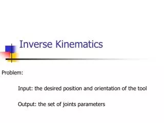
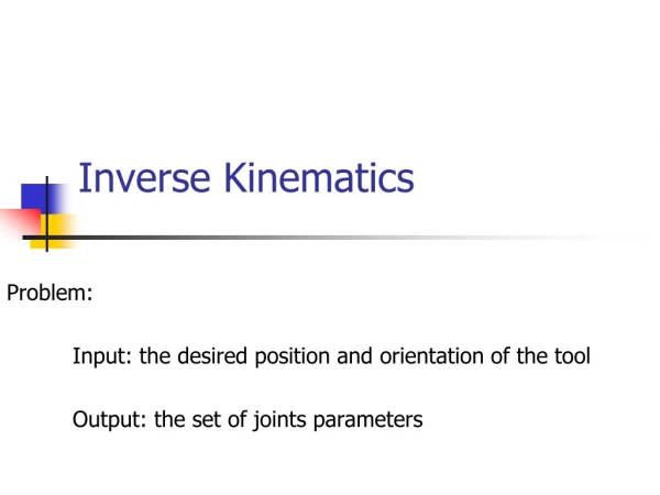
3. Forward & Inverse Kinematics • The forward kinematic function computes the world space end effector DOFs from the joint DOFs: • The goal of inverse kinematics is to compute the vector of joint DOFs that will cause the end effector to reach some desired goal state

4. Welman, 1993 • “Inverse Kinematics and Geometric Constraints for Articulated Figure Manipulation”, Chris Welman, 1993 • Masters thesis on IK algorithms • Examines Jacobian methods and Cyclic Coordinate Descent (CCD) • Please read sections 1-4 (about 40 pages)

5. Gradient Descent • We want to find the value of x that causes f(x) to equal some goal value g • We will start at some value x0 and keep taking small steps: xi+1 = xi + Δx until we find a value xN that satisfies f(xN)=g • For each step, we try to choose a value of Δx that will bring us closer to our goal • We can use the derivative to approximate the function nearby, and use this information to move ‘downhill’ towards the goal

6. Gradient Descent for f(x)=g df/dx f(xi) f-axis xi+1 g xi x-axis

7. Minimization • If f(xi)-g is not 0, the value of f(xi)-g can be thought of as an error. The goal of gradient descent is to minimize this error, and so we can refer to it as a minimization algorithm • Each step Δx we take results in the function changing its value. We will call this change Δf. • Ideally, we could have Δf = g-f(xi). In other words, we want to take a step Δx that causes Δf to cancel out the error • More realistically, we will just hope that each step will bring us closer, and we can eventually stop when we get ‘close enough’ • This iterative process involving approximations is consistent with many numerical algorithms

8. Taking Safe Steps • Sometimes, we are dealing with non-smooth functions with varying derivatives • Therefore, our simple linear approximation is not very reliable for large values of Δx • There are many approaches to choosing a more appropriate (smaller) step size • One simple modification is to add a parameter β to scale our step (0≤ β ≤1)

9. Inverse of the Derivative • By the way, for scalar derivatives:

10. Gradient Descent Algorithm

11. Jacobians • A Jacobian is a vector derivative with respect to another vector • If we have a vector valued function of a vector of variables f(x), the Jacobian is a matrix of partial derivatives- one partial derivative for each combination of components of the vectors • The Jacobian matrix contains all of the information necessary to relate a change in any component of x to a change in any component of f • The Jacobian is usually written as J(f,x), but you can really just think of it as df/dx

12. Jacobians

13. Jacobian Inverse Kinematics

14. Jacobians • Let’s say we have a simple 2D robot arm with two 1-DOF rotational joints: • e=[ex ey] φ2 φ1

15. Jacobians • The Jacobian matrix J(e,Φ) shows how each component of e varies with respect to each joint angle

16. Jacobians • Consider what would happen if we increased φ1 by a small amount. What would happen to e ? • φ1

17. Jacobians • What if we increased φ2 by a small amount? • φ2

18. Jacobian for a 2D Robot Arm • φ2 φ1

19. Jacobian Matrices • Just as a scalar derivative df/dx of a function f(x) can vary over the domain of possible values for x, the Jacobian matrix J(e,Φ) varies over the domain of all possible poses for Φ • For any given joint pose vector Φ, we can explicitly compute the individual components of the Jacobian matrix

20. Incremental Change in Pose • Lets say we have a vector ΔΦ that represents a small change in joint DOF values • We can approximate what the resulting change in e would be:

21. Incremental Change in Effector • What if we wanted to move the end effector by a small amount Δe. What small change ΔΦ will achieve this?

22. Incremental Change in e • Given some desired incremental change in end effector configuration Δe, we can compute an appropriate incremental change in joint DOFs ΔΦ Δe • φ2 φ1

23. Incremental Changes • Remember that forward kinematics is a nonlinear function (as it involves sin’s and cos’s of the input variables) • This implies that we can only use the Jacobian as an approximation that is valid near the current configuration • Therefore, we must repeat the process of computing a Jacobian and then taking a small step towards the goal until we get to where we want to be

24. Choosing Δe • We want to choose a value for Δe that will move e closer to g. A reasonable place to start is with Δe = g - e • We would hope then, that the corresponding value of ΔΦ would bring the end effector exactly to the goal • Unfortunately, the nonlinearity prevents this from happening, but it should get us closer • Also, for safety, we will take smaller steps: Δe = β(g - e) where 0≤ β ≤1

25. Basic Jacobian IK Technique while (e is too far from g) { Compute J(e,Φ) for the current pose Φ Compute J-1// invert the Jacobian matrix Δe = β(g - e) // pick approximate step to take ΔΦ = J-1·Δe// compute change in joint DOFs Φ = Φ + ΔΦ// apply change to DOFs Compute new e vector // apply forward // kinematics to see // where we ended up }

26. Computing the Jacobian

27. Computing the Jacobian Matrix • We can take a geometric approach to computing the Jacobian matrix • Rather than look at it in 2D, let’s just go straight to 3D • Let’s say we are just concerned with the end effector position for now. Therefore, e is just a 3D vector representing the end effector position in world space. This also implies that the Jacobian will be an 3xN matrix where N is the number of DOFs • For each joint DOF, we analyze how e would change if the DOF changed

28. 1-DOF Rotational Joints • We will first consider DOFs that represents a rotation around a single axis (1-DOF hinge joint) • We want to know how the world space position e will change if we rotate around the axis. Therefore, we will need to find the axis and the pivot point in world space • Let’s say φi represents a rotational DOF of a joint. We also have the offset ri of that joint relative to it’s parent and we have the rotation axis ai relative to the parent as well • We can find the world space offset and axis by transforming them by their parent joint’s world matrix

29. 1-DOF Rotational Joints • To find the pivot point and axis in world space: • Remember these transform as homogeneous vectors. r transforms as a position [rx ry rz 1] and a transforms as a direction [ax ay az 0]

30. Rotational DOFs • Now that we have the axis and pivot point of the joint in world space, we can use them to find how e would change if we rotated around that axis • This gives us a column in the Jacobian matrix

31. Rotational DOFs • a’i: unit length rotation axis in world space r’i: position of joint pivot in world space e: end effector position in world space •

32. 3-DOF Rotational Joints • For a 2-DOF or 3-DOF joint, it is actually a little trickier to get the world space axis • Consider how we would find the world space x-axis of a 3-DOF ball joint • Not only do we need to consider the parent’s world matrix, but we need to include the rotation around the next two axes (y and z-axis) as well • This is because those following rotations will rotate the first axis itself

33. 3-DOF Rotational Joints • For example, assuming we have a 3-DOF ball joint that rotates in XYZ order: • Where Ry(θy) and Rz(θz) are y and z rotation matrices

34. 3-DOF Rotational Joints • Remember that a 3-DOF XYZ ball joint’s local matrix will look something like this: • Where Rx(θx), Ry(θy), and Rz(θz) are x, y, and z rotation matrices, and T(r) is a translation by the (constant) joint offset • So it’s world matrix looks like this:

35. 3-DOF Rotational Joints • Once we have each axis in world space, each one will get a column in the Jacobian matrix • At this point, it is essentially handled as three 1-DOF joints, so we can use the same formula for computing the derivative as we did earlier: • We repeat this for each of the three axes

36. Quaternion Joints • What about a quaternion joint? How do we incorporate them into our IK formulation? • We will assume that a quaternion joint is capable of rotating around any axis • However, since we are trying to find a way to move e towards g, we should pick the best possible axis for achieving this

37. Quaternion Joints • • •

38. Quaternion Joints • We compute ai’ directly in world space, so we don’t need to transform it • Now that we have ai’, we can just compute the derivative the same way we would do with any other rotational axis • We must remember what axis we use, so that later, when we’ve computed Δφi, we know how to update the quaternion

39. Translational DOFs • For translational DOFs, we start in the same way, namely by finding the translation axis in world space • If we had a prismatic joint (1-DOF translation) that could translate along an arbitrary axis ai defined in the parent’s space, we can use:

40. Translational DOFs • For a more general 3-DOF translational joint that just translates along the local x, y, and z-axes, we don’t need to do the same thing that we did for rotation • The reason is that for translations, a change in one axis doesn’t affect the other axes at all, so we can just use the same formula and plug in the x, y, and z axes [1 0 0 0], [0 1 0 0], [0 0 1 0] to get the 3 world space axes • Note: this will just return the a, b, and c axes of the parent’s world space matrix, and so we don’t actually have to compute them!

41. Translational DOFs • As with rotation, each translational DOF is still treated separately and gets its own column in the Jacobian matrix • A change in the DOF value results in a simple translation along the world space axis, making the computation trivial:

42. Translational DOFs • •

43. Building the Jacobian • To build the entire Jacobian matrix, we just loop through each DOF and compute a corresponding column in the matrix • If we wanted, we could use more elaborate joint types (scaling, translation along a path, shearing…) and still compute an appropriate derivative • If absolutely necessary, we could always resort to computing a numerical approximation to the derivative

44. Units & Scaling • What about units? • Rotational DOFs use radians and translational DOFs use meters (or some other measure of distance) • How can we combine their derivatives into the same matrix? • Well, it’s really a bit of a hack, but we just combine them anyway • If desired, we can scale any column to adjust how much the IK will favor using that DOF

45. Units & Scaling • For example, we could scale all rotations by some constant that causes the IK to behave how we would like • Also, we could use this as an additional way to get control over the behavior of the IK • We can store an additional parameter for each DOF that defines how ‘stiff’ it should behave • If we scale the derivative larger (but preserve direction), the solution will compensate with a smaller value for Δφi, therefore making it act stiff • There are several proposed methods for automatically setting the stiffness to a reasonable default value. They generally work based on some function of the length of the actual bone. The Welman paper talks about this.

46. End Effector Orientation

47. End Effector Orientation • We’ve examined how to form the columns of a Jacobian matrix for a position end effector with 3 DOFs • How do we incorporate orientation of the end effector? • We will add more DOFs to the end effector vector e • Which method should we use to represent the orientation? (Euler angles? Quaternions?…) • Actually, a popular method is to use the 3 DOF scaled axis representation!

48. Scaled Rotation Axis • We learned that any orientation can be represented as a single rotation around some axis • Therefore, we can store an orientation as an 3D vector • The direction of the vector is the rotation axis • The length of the vector is the angle to rotate in radians • This method has some properties that work well with the Jacobian approach • Continuous and consistent • No redundancy or extra constraints • It’s also a nice method to store incremental changes in rotation

49. 6-DOF End Effector • If we are concerned about both the position and orientation of the end effector, then our e vector should contain 6 numbers • But remember, we don’t actually need the e vector, we really just need the Δe vector • To generate Δe, we compare the current end effector position/orientation (matrix E) to the goal position/orientation (matrix G) • The first 3 components of Δe represent the desired change in position: β(G.d - E.d) • The next 3 represent a desired change in orientation, which we will express as a scaled axis vector

50. Desired Change in Orientation • We want to choose a rotation axis that rotates E in to G • We can compute this using some quaternions: M=E-1·G q.FromMatrix(M); • This gives us a quaternion that represents a rotation from E to G • To extract out the rotation axis and angle, we just remember that: • We can then scale the final axis by β