Inverse Kinematics
Inverse Kinematics. Problem: Input: the desired position and orientation of the tool Output: the set of joints parameters. Workspaces. Dextrous workspace – the volume of space which the robot end-effector can reach with all orientations

Inverse Kinematics
E N D
Presentation Transcript
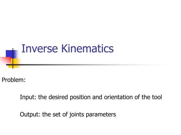
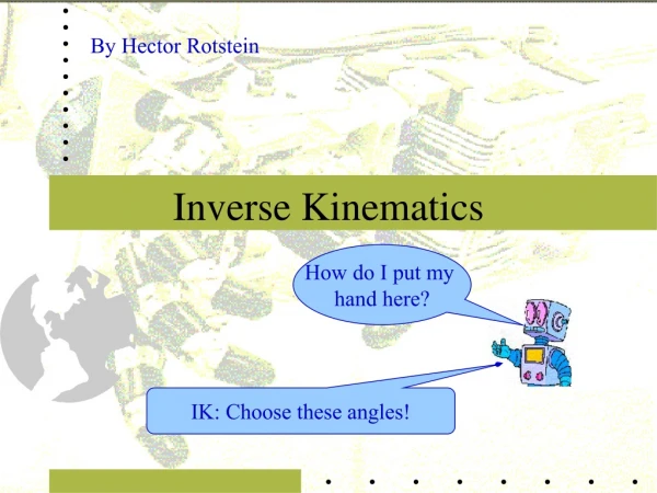
Inverse Kinematics Problem: Input: the desired position and orientation of the tool Output: the set of joints parameters
Workspaces • Dextrous workspace – the volume of space which the robot end-effector can reach with all orientations • Reachable workspace – the volume of space which the robot end-effector can reach in at least one orientation • If L1=L2then the dextrous space = {origin} and the reachable space = full disc of radius 2L1 • If then the dextrous space is empty and the reachable space is a ring bounded by discusses with radiuses |L1- L2| and L1+L2 • The dextrous space is a subset of the reachable space
Solutions • A manipulator is solvable if an algorithm can determine the joint variables. The algorithm should find all possible solutions. • There are two kinds of solutions: closed-form and numerical (iterative) • Numerical solutions are in general time expensive • We are interested in closed-form solutions: • Algebraic Methods • Geometric Methods
Algebraic Solution • Kinematics equations of this arm: • The structure of the transformation:
Algebraic Solution (cont.) • We are interested in x, y, and (of the end-effector) • By comparison of the two matrices above we obtain: • And by further manipulations: and ……
Algebraic Solution by Reduction to Polynomial • The actual variable is u :
Target • By comparison we get:
y L2 L1 x Geometric Solution IDEA: Decompose spatial geometry into several plane geometry problems 2 Applying the “law of cosines”: x2+y2=l12+l22 2l1l2cos(1802)
Geometric Solution (II) y Then: The LoC gives: l22 = x2+y2+l12 - 2l1 (x2+y2) cos So that cos = (x2+y2+l12 - l22 )/2l1 (x2+y2) We can solve for 0 180, and then 1= x