Inverse Kinematics
510 likes | 800 Views
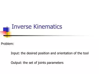
Inverse Kinematics. Robotics. "Given the desired position of the robot's hand, what must be the angles at all of the robots joints?". Animation. “How can the body of the character turn without turning his feet?. Illustration.

Inverse Kinematics
E N D
Presentation Transcript
Robotics "Given the desired position of the robot's hand, what must be the angles at all of the robots joints?"
Animation “How can the body of the character turn without turning his feet?
Illustration • Let’s say we have a simple 2D robot arm with two 1-DOF rotational joints: • e=[ex ey] φ2 φ1
Forward Kinematics • We will use the vector: to represent the array of M joint DOF values • We will also use the vector: to represent an array of N DOFs that describe the end effectors in world space.
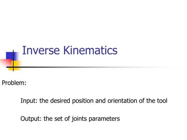
Forward & Inverse Kinematics • The forward kinematic function computes the world space end effector DOFs from the joint DOFs: • The goal of inverse kinematics is to compute the vector of joint DOFs that will cause the end effector to reach some desired goal state
Gradient Descent • We want to find the value of x that causes f(x) to equal some goal value g • We will start at some value x0 and keep taking small steps: xi+1 = xi + Δx until we find a value xN that satisfies f(xN)=g • For each step, we try to choose a value of Δx that will bring us closer to our goal • We can use the derivative to approximate the function nearby, and use this information to move ‘downhill’ towards the goal
Gradient Descent for f(x)=g df/dx f(xi) f-axis xi+1 g xi x-axis
Minimization • If f(xi)-g is not 0, the value of f(xi)-g can be thought of as an error. The goal of gradient descent is to minimize this error, and so we can refer to it as a minimization algorithm • Each step Δx we take results in the function changing its value. We will call this change Δf. • Ideally, we could have Δf = g-f(xi). In other words, we want to take a step Δx that causes Δf to cancel out the error • More realistically, we will just hope that each step will bring us closer, and we can eventually stop when we get ‘close enough’ • This iterative process involving approximations is consistent with many numerical algorithms
Taking Safe Steps • Sometimes, we are dealing with non-smooth functions with varying derivatives • Therefore, our simple linear approximation is not very reliable for large values of Δx • There are many approaches to choosing a more appropriate (smaller) step size • One simple modification is to add a parameter β to scale our step (0≤ β ≤1)
Inverse of the Derivative • By the way, for scalar derivatives:
Jacobians • A Jacobian is a vector derivative with respect to another vector • If we have a vector valued function of a vector of variables f(x), the Jacobian is a matrix of partial derivatives- one partial derivative for each combination of components of the vectors • The Jacobian matrix contains all of the information necessary to relate a change in any component of x to a change in any component of f • The Jacobian is usually written as J(f,x), but you can really just think of it as df/dx
Jacobians • Let’s say we have a simple 2D robot arm with two 1-DOF rotational joints: • e=[ex ey] φ2 φ1
Jacobians • The Jacobian matrix J(e,Φ) shows how each component of e varies with respect to each joint angle
Jacobians • Consider what would happen if we increased φ1 by a small amount. What would happen to e ? • φ1
Jacobians • What if we increased φ2 by a small amount? • φ2
Jacobian for a 2D Robot Arm • φ2 φ1
Jacobian Matrices • Just as a scalar derivative df/dx of a function f(x) can vary over the domain of possible values for x, the Jacobian matrix J(e,Φ) varies over the domain of all possible poses for Φ • For any given joint pose vector Φ, we can explicitly compute the individual components of the Jacobian matrix
Incremental Change in Pose • Lets say we have a vector ΔΦ that represents a small change in joint DOF values • We can approximate what the resulting change in e would be:
Incremental Change in Effector • What if we wanted to move the end effector by a small amount Δe. What small change ΔΦ will achieve this?
Incremental Change in e • Given some desired incremental change in end effector configuration Δe, we can compute an appropriate incremental change in joint DOFs ΔΦ Δe • φ2 φ1
Incremental Changes • Remember that forward kinematics is a nonlinear function (as it involves sin’s and cos’s of the input variables) • This implies that we can only use the Jacobian as an approximation that is valid near the current configuration • Therefore, we must repeat the process of computing a Jacobian and then taking a small step towards the goal until we get to where we want to be
Choosing Δe • We want to choose a value for Δe that will move e closer to g. A reasonable place to start is with Δe = g - e • We would hope then, that the corresponding value of ΔΦ would bring the end effector exactly to the goal • Unfortunately, the nonlinearity prevents this from happening, but it should get us closer • Also, for safety, we will take smaller steps: Δe = β(g - e) where 0≤ β ≤1
Basic Jacobian IK Technique while (e is too far from g) { Compute J(e,Φ) for the current pose Φ Compute J-1// invert the Jacobian matrix Δe = β(g - e) // pick approximate step to take ΔΦ = J-1·Δe// compute change in joint DOFs Φ = Φ + ΔΦ// apply change to DOFs Compute new e vector // apply forward // kinematics to see // where we ended up }
Inverting the Jacobian • If the Jacobian is square (number of joint DOFs equals the number of DOFs in the end effector), then we might be able to invert the matrix • Most likely, it won’t be square, and even if it is, it’s definitely possible that it will be singular and non-invertable • Even if it is invertable, as the pose vector changes, the properties of the matrix will change and may become singular or near-singular in certain configurations • The bottom line is that just relying on inverting the matrix is not going to work
Underconstrained Systems • If the system has more degrees of freedom in the joints than in the end effectors, then it is likely that there will be a continuum of redundant solutions (i.e., an infinite number of solutions) • In this situation, it is said to be under constrained or redundant • These should still be solvable, and might not even be too hard to find a solution, but it may be tricky to find a ‘best’ solution
Overconstrained Systems • If there are more degrees of freedom in the end effectors than in the joints, then the system is said to be over constrained, and it is likely that there will not be any possible solution • In these situations, we might still want to get as close as possible • However, in practice, over constrained systems are not as common, as they are not a very useful way to build an animal or robot (they might still show up in some special cases though)
Well-Constrained Systems • If the number of DOFs in the end effector equals the number of DOFs in the joints, the system could be well constrained and invertable • In practice, this will require the joints to be arranged in a way so their axes are not redundant • This property may vary as the pose changes, and even well-constrained systems may have trouble
Pseudo-Inverse • If we have a non-square matrix arising from an over constrained or under constrained system, we can try using the pseudo inverse: J*=(JTJ)-1JT • This is a method for finding a matrix that effectively inverts a non-square matrix
Single Value Decomposition • The SVD is an algorithm that decomposes a matrix into a form whose properties can be analyzed easily • It allows us to identify when the matrix is singular, near singular, or well formed • It also tells us about what regions of the multidimensional space are not adequately covered in the singular or near singular configurations • The bottom line is that it is a more sophisticated, but expensive technique that can be useful both for analyzing the matrix and inverting it
Iteration • Whether we use the JI, JP, or JT method, we must address the issue of iteration towards the solution • We should consider how to choose an appropriate step size β and how to decide when the iteration should stop
When to Stop • There are three main stopping conditions we should account for • Finding a successful solution (or close enough) • Getting stuck in a condition where we can’t improve (local minimum) • Taking too long (for interactive systems) • All three of these are fairly easy to identify by monitoring the progress of Φ • These rules are just coded into the while() statement for the controlling loop
Finding a Successful Solution • We really just want to get close enough within some tolerance • If we’re not in a big hurry, we can just iterate until we get within some floating point error range • Alternately, we could choose to stop when we get within some tolerance measurable in pixels • For example, we could position an end effector to 0.1 pixel accuracy • This gives us a scheme that should look good and automatically adapt to spend more time when we are looking at the end effector up close (level-of-detail)
Local Minima • If we get stuck in a local minimum, we have several options • Don’t worry about it and just accept it as the best we can do • Switch to a different algorithm (CCD…) • Randomize the pose vector slightly (or a lot) and try again • Send an error to whatever is controlling the end effector and tell it to try something else • Basically, there are few options that are truly appealing, as they are likely to cause either an error in the solution or a possible discontinuity in the motion
Taking Too Long • In a time critical situation, we might just limit the iteration to a maximum number of steps • Alternately, we could use internal timers to limit it to an actual time in seconds
Iteration Stepping • Step size • Stability • Performance
Joint Limits • A simple and reasonably effective way to handle joint limits is to simply clamp the pose vector as a final step in each iteration • One can’t compute a proper derivative at the limits, as the function is effectively discontinuous at the boundary • The derivative going towards the limit will be 0, but coming away from the limit will be non-zero. This leads to an inequality condition, which can’t be handled in a continuous manner • We could just choose whether to set the derivative to 0 or non-zero based on a reasonable guess as to which way the joint would go. This is easy in the JT method, but can potentially cause trouble in JI or JP
Higher Order Approximation • The first derivative gives us a linear approximation to the function • We can also take higher order derivatives and construct higher order approximations to the function • This is analogous to approximating a function with a Taylor series
Repeatability • If a given goal vector g always generates the same pose vector Φ, then the system is said to be repeatable • This is not likely to be the case for redundant systems unless we specifically try to enforce it • If we always compute the new pose by starting from the last pose, the system will probably not be repeatable • If, however, we always reset it to a ‘comfortable’ default pose, then the solution should be repeatable • One potential problem with this approach however is that it may introduce sharp discontinuities in the solution
Multiple End Effectors • Remember, that the Jacobian matrix relates each DOF in the skeleton to each scalar value in the e vector • The components of the matrix are based on quantities that are all expressed in world space, and the matrix itself does not contain any actual information about the connectivity of the skeleton • Therefore, we extend the IK approach to handle tree structures and multiple end effectors without much difficulty • We simply add more DOFs to the end effector vector to represent the other quantities that we want to constrain • However, the issue of scaling the derivatives becomes more important as more joints are considered
Multiple Chains • Another approach to handling tree structures and multiple end effectors is to simply treat it as several individual chains • This works for characters often, as we can animate the body with a forward kinematic approach, and then animate each limb with IK by positioning the hand/foot as the end effector goal • This can be faster and simpler, and actually offer a nicer way to control the character
Geometric Constraints • One can also add more abstract geometric constraints to the system • Constrain distances, angles within the skeleton • Prevent bones from intersecting each other or the environment • Apply different weights to the constraints to signify their importance • Have additional controls that try to maximize the ‘comfort’ of a solution
Other IK Techniques • Cyclic Coordinate Descent • This technique is more of a trigonometric approach and is more heuristic. It does, however, tend to converge in fewer iterations than the Jacobian methods, even though each iteration is a bit more expensive • Analytical Methods • For simple chains, one can directly invert the forward kinematic equations to obtain an exact solution. This method can be very fast, very predictable, and precisely controllable. With some finesse, one can even formulate good analytical solvers for more complex chains with multiple DOFs and redundancy • Other Numerical Methods • There are lots of other general purpose numerical methods for solving problems that can be cast into f(x)=g format