Download
1 / 64
640 likes | 660 Views
NTU, Taida Institute for Mathematical Sciences (TIMS) November 4 th , 2015. Including groundwater in land surface models for hydrologic and climatic applications. Agnès DUCHARNE Senior scientist at CNRS (Centre National de la Recherche Scientifique)

E N D
NTU, Taida Institute for Mathematical Sciences (TIMS) November 4th, 2015 Including groundwater in land surface models for hydrologic and climatic applications Agnès DUCHARNE Senior scientist at CNRS (Centre National de la Recherche Scientifique) METIS Laboratory, Université Pierre et Marie Curie, Paris Agnes.Ducharne@upmc.fr
Outline • Introduction: what are land surface models (LSMs) ? • and why groundwater (GW) may be important ? • GW effect on surface hydrology: with the Catchment LSM • GW effect on climate: with the ORCHIDEE LSM • Perspectives
1. Introduction Why is the land surface important? • We live there ! • Interface betweenatmosphere and underground domain, with a lot of spatial heterogeneities • Involved in the climate system by means of mass, energy, and momentum fluxes
1. Introduction Land surface models (LSMs) • First developed as components of climatemodels: • Ocean model • Sea-ice model • Atmosphericmodel • Land surface model • LW↑ SW↑ • H λE Hydrology Image D. Vischer
1. Introduction LSM history SVAT models e.g. Sellers et al. (1986) Third generation « Bucket » model Manabe (1969) Improving hydrological processes: soil properties, runoff generation processes, GW Beyond water and energy fluxes: carbon cycle, N cycle, vegetation dynamics From climate models to Earth system models 1 0 W/Wmax 0 1
1. Introduction Definitions around GW • Soil moisture (SM) • Water table (WT) • Ground water (GW) • 25% of total global freshwater withdrawals come from GW/aquifers (Margat & van der Gun, 2013)
1. Introduction GW flows ! PL • Baseflow (Qb) • R or Q: runoff or liquid water flow • ET: evapotranspiration • P: precipitation ET Q Mean annual fluxes of the global water cycle (103 km3 yr−1) during 2000-2010. White numbers are based on observational products and data integrating models. Blue numbers have been optimized by forcing water and energy budget closure, taking into account uncertainty in the original estimates. Rodell et al., 2015
1. Introduction Buffering effects of GW Hydrology point of view: buffer effect on streamflow From MH Lo, after Entekhabi et al. (1996)
1. Introduction Buffering effects of GW ? Climate point of view: buffer effect on SM, ET, P From MH Lo, after Entekhabi et al. (1996)
1. Introduction The crucial role of water table depth (WTD) • GW is not a simple object • Just looking at WT, their depth can vary a lot (temporally and spatially) Mean observed WTD in the US (Gascoin, 2009; after Fan et al., 2007) < 5m (34 %) > 5m (66 %)
1. Introduction Classifying the water table at regional to continental scales(Gleeson et al, 2011) The crucial role of water table depth (WTD) • GW is not a simple object • Just looking at WT, their depth can vary a lot (temporally and spatially) • Their other properties can also vary a lot (thickness, porosity, permeability, etc.) (b) recharge controlled WT (a) topography‐controlled WT
Outline • Introduction: what are land surface models (LSMs) ? • and why may groundwater (GW) be important ? • GW effect on surface hydrology: with the Catchment LSM • Model summary • Two «off-line» studies in Northern France • GW effect on climate: with the ORCHIDEE LSM • Perspectives
2. GW effect on surface hydrology The Catchment LSM • Developed @ NASA/GSFC by Koster et al. (2000) & Ducharne et al. (2000) • For climate models, but calculation units are catchments instead of regular grid-cells • Enables using the concepts of hydrologic model TOPMODEL (Beven & Kirkby, 1979)
2. GW effect on surface hydrology TOPMODEL • Topographicallydriven WT hydraulic gradient = topographicslope • Qb : BaseflowDarcy law (saturated flow) KS= K0exp(-νz) • QS : Surface runoffFromsaturated areas • Topographic index • Index of wetnesspotential • Index of similarity • ln(a/tanβ) 20 2 a : upstream contributing area tanβ : local slope
2. GW effect on surface hydrology TOPMODEL Topographic index • Topographicallydriven WT hydraulic gradient = topographicslope • Qb : BaseflowDarcy law (saturated flow) KS= K0exp(-νz) • QS : Surface runoffFromsaturated areas density
2. GW effect on surface hydrology TOPMODEL Topographic index • Topographicallydriven WT hydraulic gradient = topographicslope • Qb : BaseflowDarcy law (saturated flow) KS= K0exp(-νz) • QS : Surface runoffFromsaturated areas density WTD (m) density
2. GW effect on surface hydrology TOPMODEL Topographic index • Topographicallydriven WT hydraulic gradient = topographicslope • Qb : BaseflowDarcy law (saturated flow) KS= K0exp(-νz) • QS : Surface runoffFromsaturated areas densité WTD (m) densité
2. GW effect on surface hydrology TOPMODEL Topographic index • Topographicallydriven WT hydraulic gradient = topographicslope • Qb : BaseflowDarcy law (saturated flow) KS= K0exp(-νz) • QS : Surface runoffFromsaturated areas density WTD (m) density
2. GW effect on surface hydrology The Catchment LSM Uses the above concepts, via non traditional state variables to: • Calculate the runoffterms • Definethreeareal fractions, withdifferent SM thus stress factors on ET • These fractions varywithbulkmoisture • ln(a/tanβ) stressed transpiring saturated
2. GW effect on surface hydrology The Catchment LSM SM states variables: 1. The catchment deficit (a) Given a local WTD, we define a vertical equilibrium profile (hydrostatic) local SM deficit Wetness Unsaturated zone Equilibrium profile WTD (b) Horizontal integration of the local deficit along the WTD distribution
2. GW effect on surface hydrology The Catchment LSM SM states variables: 2. Excess variables Net infiltration Net exfiltration Surface excess Root zone Root zone RZ excess • Surface and RZ excess: • influence transpiration, soil evaporation, surface runoff • are linked to the «vertical» fluxes and mean WTD variations
2. GW effect on surface hydrology The Somme river basin • Surface @ Abbeville = 5,560 km² • Mostly embedded in the Chalk aquifer • Feeds 90% of streamflow (BRGM) • Free WT • Mean WTD = 40 m • Recharge-controlled Source : F. Habets Main aquifer formations
2. GW effect on surface hydrology The Somme river basin Streamflow @ Abbeville [m3/s] Abbeville, April 10, 2001 • CLSM performscorrectly • 5-6 yrperiodicityrelated to NAO • + GW memory • Centenial flood in 2001 Abbeville le 10 avril 2001 (Photo AFP)
2. GW effect on surface hydrology Is CLSM adapted? Original version: 1985 1987 1989 1991 1993 1995 1997 1999 2001 2003 Various parameter tuning were tested: • Ks , • Ks anisotropy • Soil depth to bedrock Not sucessfull
2. GW effect on surface hydrology CLSM modification G Original CLSM CLSM-LR Similarities with CLM but no upward capillary flux from the « aquifer »
2. GW effect on surface hydrology Result Best CLSM vs. Best CLSM-LR (τG = 700 jours) Gascoin et al. (2009)
2. GW effect on surface hydrology The Seine river basin • Surface @ Poses = 66,710 km² • Mostlyembedded in the Chalkaquifer • Feeds up to 80% of streamflow • Stronghuman pressures • Urbanization in river corridors Source : F. Habets Main aquifer formations
2. GW effect on surface hydrology The Seine river basin • Surface @ Poses = 66,710 km² • Mostlyembedded in the Chalkaquifer • Feeds up to 80% of streamflow • Stronghuman pressures • Urbanization in river corridors • Intensive agriculture Source : F. Habets Main aquifer formations
2. GW effect on surface hydrology The Seine river basin • Surface @ Poses = 66,710 km² • Mostlyembedded in the Chalkaquifer • Feeds up to 80% of streamflow • Stronghuman pressures • Urbanization in river corridors • Intensive agriculture • Whichvulnerability to climate change? Source : F. Habets Main aquifer formations
2. GW effect on surface hydrology Climate change impact assessment Annual means GHG scenarios (2) Climatemodels (15) Large-scale climate projections Downscaling and bias correction (3) Regionalized climate projections • P: -6% in 2050; -12%in 2100 • PET: + 16% in 2050; + 23 %in 2100 Hydrologicmodels (5) The climatebecomesdrier Uncertainties Hydrologic projections
2. GW effect on surface hydrology The CLSM response is very strong • CLSM in orange • Only model withincreasing ET • Largest Q decrease Ducharne et al. (2009)
2. GW effect on surface hydrology The CLSM response is very strong 2000 2050 Habets et al. (2013) 2100 • The WT has a tighthydraulicconnectionwith the soil • (despite the LR reservoir) • This sustainslarger SM seasonal variations, • and larger ET at the beginning of summer
2. GW effect on surface hydrology This behavior is likely excessive Based on observations of TWS anomalies in Eastern France Loessic hill (Hausbergen, Alsace) Severe heat wave and drought in summer 2003 Longuevergne et al., 2012
2. GW effect on surface hydrology Conclusions about the CLSM • Pioneering model with full couplingbetween WT and SM, withsimplified 2D flow and sub-basin variability of SM and surface fluxes • Based on a model for topography-driven WT • (TOPMODEL) needs adaptation for deeper, • lowhydraulic gradient aquifers • In dry conditions, the capillaryriseistoostrong • and lowers the GW bufferingeffect on ET and Q
Outline • Introduction: what are land surface models (LSMs) ? • and why may groundwater (GW) be important ? • GW effect on surface hydrology: with the Catchment LSM • GW effect on climate: with the ORCHIDEE LSM • Model summary • One «on-line» study at two scales in Europe • Perspectives
3. GW effect on climate The ORCHIDEE LSM Atmosphere Prescribed or Modeled (using LMDZ) Ta, qa, wind, P, incoming radiation, pressure CO2 concentration H, LE, Ts, albedo, roughness, net radiation CO2 fluxes Energy and Water Budgets with options for Photosynthesis and Routing SECHIBA (t = 30 min) GPP, soil profiles of temperature and water LAI, albedo, roughness LMDZOR or IPSL-CM if ocean / sea-ice models Vegetation and Soil Carbon Cycle with options for N cycle, etc. STOMATE (t =1 day) NPP, biomass, litterfall, etc. vegetation types Vegetation distribution Prescribed or Modeled (using LPJ DGVM) t =1 year
3. GW effect on climate Soil hydrology in ORCHIDEE E • 1D soil water fluxes based on Richards equation (unsaturated flow) • 2-m soiland 11-layers • Hydraulic properties based on van Genuchten-Mualem formulation • Related parameter based on texture (fine, medium, coarse) • Infiltration depends on precipitation rate • Surface runoff = P – Esoil – Infiltration • Free drainage at the bottom • No GW P Rs de Rosnay et al., 2002; d’Orgeval et al., 2008 D
3. GW effect on climate Comparison to observation in coupled mode Multi-instrumented observatory SIRTA LMDZOR zoomed and nudged c Precipitation rate @ SIRTA observatory – Summer 2009 Cheruy et al., 2012
3. GW effect on climate Comparison to observation in coupled mode Température de l’air à 2 m (°C) Flux de chaleur latente (W/m²) OBS REF Campoy et al., 2011
3. GW effect on climate Comparison to observation in coupled mode • OBS • REF Shallow WTD at SIRTA Not reproduced, by far, by ORCHIDEE Saturation
3. GW effect on climate How to increase ORCHIDEE’s realism? Preliminary adjustments of the code
3. GW effect on climate Impact of prescribed WTD: surface variables REF
3. GW effect on climate Impact of prescribed WTD: atmospheric variables Differenceswith REF Plain lines: Local WTD forcing (SIRTA grid-cell) Dasheslines: Global WTD forcing Strongereffect if global forcing Especially for P
3. GW effect on climate Water cycle in Europe E [mm/d] x REF GF0.00 No drainage GS1.3 Fixed WT at 1.3m Campoy et al., 2013
3. GW effect on climate Water cycle in Europe GW effect on E in CESM Lo et Famiglietti, 2011 E [mm/d] • The effect of increased SM on ET increasessouthward: • ET energylimited at higher latitudes • ET more & more SM limitedsouthward Campoy et al., 2013
3. GW effect on climate Water cycle in Europe E [mm/d] Over Eastern Europe, P more than E, owing to moisture convergence (from the West) Over Western Europe, it’s the opposite Over Southern Europe, P also less than E, as air is too dry P [mm/d] P-E [mm/d] Campoy et al., 2013
Outline • Introduction: what are land surface models (LSMs) ? • and why may groundwater (GW) be important ? • GW effect on surface hydrology: with the Catchment LSM • GW effect on climate: with the ORCHIDEE LSM • Perspectives
4. Perspectives ANR-MoST project I-GEM = Impact of Groundwater in Earth system Models2014-2018 France/IPSL/Paris: Agnès DUCHARNE (co-PI) Frédérique CHERUY Jan POLCHER Anne JOST Fuxing WANG (IGEM post-doc) Ana SCHNEIDER (PhD student) Ardalan TOOTCHI (PhD student) Taiwan / NTU: Lo, Min-Hui (co-PI) Chien, Rong-You (research assistant) Wu, Ren-Jie (research assistant) Wu, Wen-Ying (research assistant) Lan, Chia-Wei (PhD student) France/CNRM/Toulouse: Bertrand DECHARME Jeanne COLIN Sophie TYTECA
4. Perspectives ANR-MoST project
4. Perspectives GW in ORCHIDEE – 1. Runoff routing Cascade of linear reservoirs along the river network Separate reservoirs for streams, hillslopes and GW Basin Q1out Qin Qout g1 1 Surface Runoff Q2out g2 2 Drainage Q3out g3 3 Polcher 2003; Guimberteau et al., 2012